Which model when?¶
Start from your problem, not from a method. This is the flagship entry point to tsecon: you arrive with a symptom — "my series won't hold still", "I have quarterly GDP and monthly indicators", "my regressor is nearly a unit root" — and each section routes you to the function that answers it, tells you in one line when it applies, shows the exact call, and links to the guide chapter and gallery figure that go deeper.
Every path ends at a real, shipped function. Where the honest answer is "not yet — that's on the roadmap", the section says so and names the closest thing that ships today rather than pretending. Every code block below was run against the library before publication; the tricky ones read their inputs from the repository's golden fixtures so you can reproduce them from the repository root.
A word on shapes, because it is the most common stumbling block. tsecon is consistent but opinionated about array layout:
- a single series is a 1-D array of length
T; - a system (VAR, connectedness, cointegration, factors, yield-curve panel)
is
T × k— time down the rows, variables across the columns; - a panel for the fixed-effects/mean-group family is
N × Tfor the outcome andk × N × Tfor regressors; the heterogeneous-panel estimators (panel_mean_group,panel_pmg) instead take Python lists of per-unit arrays, because unitimay have its own lengthT_i.
When a call complains about dimensions, it is almost always this.
The decision table¶
Not sure where to start? tsecon.check_series(y) is this page as an
executable: one call runs the diagnostic families and returns recommendations
that route to the same functions the rows below name (see the
model card). Run it first, then come
back here for the branches it cannot see — it inspects one dataset; it cannot
know your research question.
A compact index. Find your row, jump to the section.
| Your situation | Reach for | Section |
|---|---|---|
| Series may be nonstationary; need to decide whether to difference | check_stationarity (adf + kpss) |
1 |
| Unit-root test without picking an augmentation lag (ADF alternative / cross-check) | phillips_perron |
1 |
| Is a price (log level) a random walk — are its increments serially uncorrelated, robust to volatility clustering? | variance_ratio (Lo-MacKinlay; a list of horizons adds the Chow-Denning joint test) |
1 |
| Impulse response, and you trust a recursive ordering | var_irf (var_fit, var_fevd) |
2 |
| Impulse response, but you only trust the signs of a few responses | sign_restricted_svar |
2 |
| Impulse response combining exact zeros with sign restrictions | zero_sign_svar (RWZ 2010 + ARW 2018) |
2 |
| Impulse response with a long-run neutrality (permanent vs transitory) | long_run_svar (Blanchard-Quah) |
2 |
| The single shock that drives a target's business-cycle variance | max_share_svar (main-BC / news shock) |
2 |
| Impulse response from one measured instrument / narrative surprise | proxy_svar (SVAR-IV) |
2 |
| Impulse response from documented variance regimes (crisis vs calm) | hetero_svar (Rigobon) |
2 |
| Impulse response with no defensible sign/zero restriction, but plausibly non-Gaussian shocks | nongaussian_svar (independent-component / ICA) |
2 |
| Variance decomposition (FEVD) for an already-identified shock (any scheme) | structural_fevd |
2 |
| How much did shock j contribute to variable i in episode X | historical_decomposition |
2 |
| One coherent IRF from a sign-restricted set (not the median-mixes-models band) | fry_pagan_svar (median-target) |
2 |
| Sign-restriction bounds with the Haar-prior artifact removed | robust_svar_bounds (Giacomini-Kitagawa) |
2 |
| Shrink a sign-identified set with knowledge of a historical episode | narrative_svar (Antolín-Díaz-Rubio-Ramírez) |
2 |
| A Bayesian VAR that selects which coefficients are non-zero | bvar_ssvs (spike-and-slab SSVS) |
2 |
| Impulse response from one equation, no full VAR to commit to | lp; instrumented lp_iv; state-dependent lp_state — LP or VAR? chapter 16 measures it |
2 |
| Quarterly target, monthly indicators, a ragged data edge | dfm_nowcast |
3 |
| A handful of high-frequency lags to compress into a target | weighted_midas (large ratio) / umidas (small ratio) / adl_midas (persistent target: adds its own lags) |
3 |
| Volatility with fat tails or occasional jumps | gas_volatility(density="student_t") |
4 |
| Intraday returns / a realized-variance series | realized_measures, har_rv |
4 |
| Panel whose units have genuinely different slopes | panel_mean_group (mg/cce), panel_pmg |
5 |
| Is a whole panel of series I(1)? (pre-test before a panel VAR / cointegration) | panel_unit_root (LLC / IPS / Fisher) |
5 |
| A fiscal (integral) multiplier from an instrumented shock | lp_multiplier — not lp_iv(..., cumulative=True) |
2 |
| A smoother, lower-variance IRF across horizons | smooth_lp (B-spline penalty; λ=0 = raw LP) |
2 |
| The shock is a whole curve (e.g. the yield curve shifts) | functional_pca + flp_scenario / fvar_scenario |
2 |
| Downside risk of growth, not the mean forecast | growth_at_risk (conditional quantiles, ABG) |
4 |
| The whole IRF at a tail quantile (downside dynamics, not the mean path) | quantile_lp; static coefficients quantile_regression |
4 |
| Did the coefficients break, and how many times? | bai_perron (unknown, multiple), sup_f_test (unknown, single); known date chow_test |
1 |
| Panel IRF to a common shock; per-entity dynamics | panel_lp, mean_group_var |
5 |
| Panel with a time-invariant regressor of interest (FE cannot estimate it) | panel_re — after the Mundlak check |
5 |
| FE or RE? | the Mundlak check: entity means as extra panel_re regressors, Wald on their cov |
5 |
| Cross-sectional (asset-pricing) regressions, period by period | panel_fama_macbeth |
5 |
| Regressor is highly persistent (predictive regression) | predictive_regression (OLS + Stambaugh + IVX), ivx_test |
6 |
| Many candidate predictors, most of them noise | adaptive_lasso, lasso_path, cv_splits |
7 |
| Spillovers / who-shocks-whom across many markets | connectedness |
8 |
| Single-equation cointegration test (is this pair tied in the long run?) | phillips_ouliaris; rank via johansen |
8 |
| Is there a level relationship, when the regressors may be I(0) or I(1)? | ardl_bounds_test (Pesaran-Shin-Smith bounds) |
8 |
| Fit or forecast a yield curve | nelson_siegel, svensson, dynamic_ns |
9 |
| Endogenous regressor with instruments | iv_gmm; nonlinear moments gmm_nonlinear |
10 |
Two cross-cutting escape hatches used throughout: robust standard errors
(se_type="hac" on any regression estimator, and ols(se_type="ewc") —
Student-t_B p-values — when size matters with persistent errors; see
chapter 3) and honest out-of-sample
evaluation (backtest, dm_test; see chapter 5).
Never report an estimate without the first or a forecast without the second.
1 · Is my series stationary? Do I need to difference?¶
The question in plain words: before you fit anything, does the series revert to a stable mean, or does it wander like a random walk? Get this wrong and every downstream standard error is a fiction.
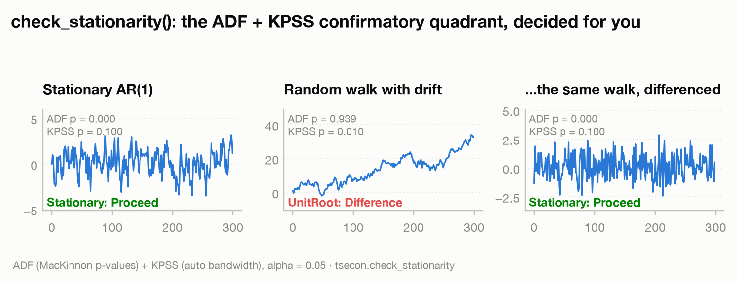
The decision path. Do not run one test. The ADF null is a unit root; the
KPSS null is stationarity — they answer complementary questions, and only
together do they give a confident verdict. check_stationarity runs both and
reports the confirmatory quadrant plus a recommendation.
import numpy as np, tsecon

rng = np.random.default_rng(0)
y = np.cumsum(rng.standard_normal(300))          # a random walk

rep = tsecon.check_stationarity(y)
rep["recommendation"]   # -> "Difference"
rep["quadrant"]         # -> "UnitRoot"  (both tests agree)
- Both tests agree it's a unit root (
quadrant="UnitRoot", recommendation"Difference") — difference the series and re-test the difference. - Both agree it's stationary (
"Stationary","Proceed") — proceed to modeling on the level. - They conflict (
"Conflict"/"Inconclusive") — the series may be trend-stationary or have a break; detrend, or reach for the individual tests and inspect the regression option.
Run the components directly when you need the statistic and p-value:
tsecon.adf(y, regression="c")["p_value"]         # ADF, constant only
tsecon.kpss(y, regression="ct")["p_value"]       # KPSS around a linear trend
Prefer not to pick an augmentation lag? phillips_perron is the
semiparametric alternative to ADF: it runs the plain Dickey-Fuller level
regression and corrects the statistic for serial correlation with a kernel long-run
variance instead of adding lagged differences. Same unit-root null, same MacKinnon
p-values, no maxlag to choose. Use it as a robustness cross-check on ADF —
agreement between the two is reassuring — but it shares ADF's low power near the
boundary, so it does not replace the ADF+KPSS quadrant.
pp = tsecon.phillips_perron(y, regression="c")   # test_type="tau" (Z-tau) or "rho" (Z-alpha)
pp["stat"], pp["pvalue"], pp["lags"]             # small p ⇒ reject the unit root
A unit root is not yet a random walk. Once the level is I(1), the next
question — the market-efficiency one for a log price — is whether its
increments are serially uncorrelated. variance_ratio (Lo-MacKinlay) compares
the variance of q-period changes with q times the one-period variance: 1 under a
random walk, above 1 under momentum, below 1 under mean reversion. Its default
statistic is robust to volatility clustering, which Ljung-Box on the returns is
not. Pass the LEVEL series, not returns; a list of horizons adds the Chow-Denning
joint test:
vr = tsecon.variance_ratio(y, lags=[2, 4, 8, 16])   # y = log prices (levels)
vr["vr"], vr["pvalue"]                             # per horizon
vr["cd_stat"], vr["cd_pvalue"]                     # one joint verdict across horizons
Escape hatch — did the relationship break? A conflict that survives
detrending often means a structural break: the mean, or a regression
coefficient, moved once rather than every period. Do not eyeball it — test for
it. With a known candidate date, chow_test(y, X, split) is the textbook
F-test. When the date is unknown, sup_f_test scans every interior date and
returns the strongest break with a Hansen (1997) p-value; bai_perron goes
further and estimates how many breaks there are (sequential supF(l+1|l)) with a
confidence interval on each date:
import numpy as np, tsecon

rng = np.random.default_rng(0); T = 200
X = np.column_stack([np.ones(T), rng.standard_normal(T)])     # regressors; ALL coefficients may switch
b1, b2 = np.array([0.0, 0.5]), np.array([2.0, 0.5])           # the intercept jumps at t=100
yb = np.empty(T)
yb[:100] = X[:100] @ b1 + rng.standard_normal(100) * 0.5
yb[100:] = X[100:] @ b2 + rng.standard_normal(100) * 0.5

sf = tsecon.sup_f_test(yb, X)                     # unknown single break
sf["stat"], sf["p_value"], sf["break_date"]       # reject the null of stability ⇒ break at break_date
bp = tsecon.bai_perron(yb, X, max_breaks=3)       # unknown, possibly several
bp["n_breaks"], bp["break_dates"], bp["ci_lower_95"], bp["ci_upper_95"]
ch = tsecon.chow_test(yb, X, split=100)           # a *known* candidate date
ch["fstat"], ch["pvalue"]
To watch parameters drift rather than count discrete breaks,
cusum_test(yb, X) returns the recursive-residual CUSUM path and its 5% bounds.
If two series are each I(1) but move together, you do not want to difference away their shared trend — that is cointegration, section 8.
Go deeper: chapter 2 — KPSS and the confirmatory quadrant · gallery figure
2 · I want an impulse response¶
The question in plain words: the system gets hit by a shock — how do the variables respond over the following quarters? This is the workhorse question of empirical macro, and the right tool depends entirely on what identifying assumption you are willing to defend. That is the fork below.
2a · …and I trust a recursive (Cholesky) ordering¶
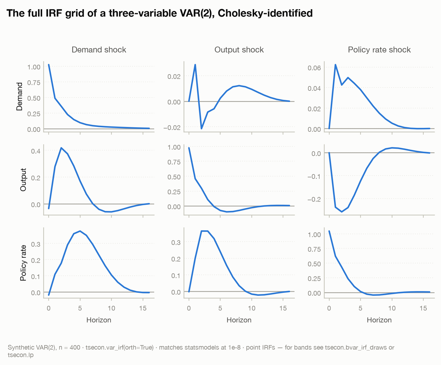
When it applies: you can order the variables so that each one responds to the shocks above it only with a lag — the classic "slow" real block, then a "fast" financial block. The ordering is your identifying assumption; own it.
import json, numpy as np, tsecon

data = np.array(json.load(open("fixtures/var.json"))["data_100dlog_gdp_cons_inv"])  # T x 3

fit  = tsecon.var_fit(data, lags=2)                       # coefficients, ICs, stability
fit["is_stable"]                                           # True ⇒ stable (read this)
fit["min_root"]                                            # > 1 ⇒ stable (reciprocal roots)

irf  = tsecon.var_irf(data, lags=2, horizon=16, orth=True)   # [h][response][shock]
fevd = tsecon.var_fevd(data, lags=2, horizon=16)             # variance decomposition
Check fit["is_stable"] before you trust any IRF — an explosive VAR has no
meaningful impulse response. (The roots are the reciprocal characteristic
roots, so stability means every modulus exceeds 1, i.e. min_root > 1.
max_root is the root farthest from the unit circle and stays above 1 even for
an explosive system, so it is not a verdict on its own.) orth=True applies the Cholesky factorization in
column order; reorder the columns to change the ordering assumption.
Put a band on it. A point IRF invites over-reading; report the uncertainty.
Frequentist bands come from var_irf_bands — Lütkepohl (1990) delta-method
(method="asymptotic") or a Kilian (1998) residual bootstrap
(method="bootstrap"), with the same orth/cumulative flags as var_irf.
Bayesian credible bands come from bvar_irf_draws (the escape hatch below);
set-identified bands under sign restrictions from sign_restricted_svar
(2b).
band = tsecon.var_irf_bands(data, lags=2, horizon=16, orth=True, method="asymptotic", alpha=0.1)
lo, hi = np.asarray(band["lower"]), np.asarray(band["upper"])
lo[1, 1, 0], hi[1, 1, 0]        # (0.030, 0.184): 90% band, consumption's h=1 response to a GDP shock
The var_irf_bands bands are pointwise (one horizon at a time), not joint
over the whole path — the honest per-horizon uncertainty, not a simultaneous
coverage statement.
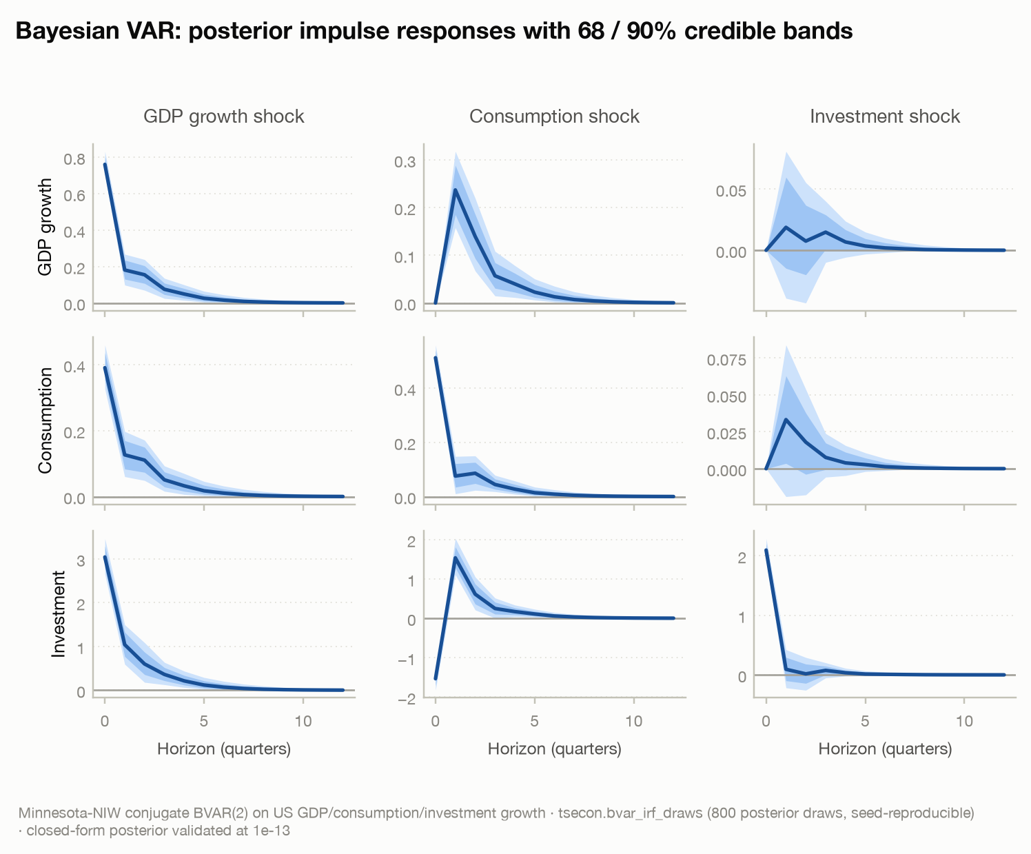
Escape hatch — short sample, noisy IRFs. Macro samples are short and VARs are parameter-hungry, so the frequentist IRF can be jagged. Shrink it with a Minnesota-prior Bayesian VAR and read credible bands off posterior draws:
draws = tsecon.bvar_irf_draws(data, lags=2, horizon=12, n_draws=200, seed=42)
bands = np.quantile(draws, [0.05, 0.5, 0.95], axis=0)     # [draw][h][var][shock]
See chapter 10 — the conjugate NIW-BVAR
and its gallery figure. If instead you suspect the
system is sparse — most distant lags and cross-effects truly zero — let the
data select which coefficients survive with bvar_ssvs (spike-and-slab
stochastic search): it returns a posterior inclusion probability per
coefficient plus the same Cholesky-IRF draws for bands.
ss = tsecon.bvar_ssvs(data, lags=2, n_draws=4000, burn=1000, seed=1, n_chains=2)
ss["inclusion_prob"]                   # per-coefficient posterior inclusion (intercept row = 1)
ss["diagnostics"]["rhat"]              # < 1.01 to trust it (needs n_chains >= 2)
Go deeper: chapter 7 — IRFs and FEVD · chapter 8 — recursive identification · gallery figure
2b · …but I only trust sign restrictions¶
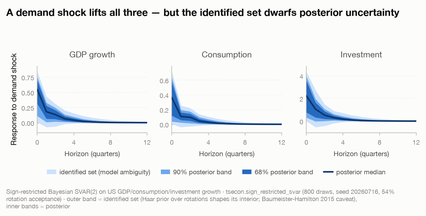
When it applies: you cannot defend an ordering, but theory does tell you the sign of a few impact responses ("a demand shock raises output, consumption, and investment on impact"). Sign restrictions ask for exactly that and return the whole identified set — every response consistent with the signs — not a single line.
restr = [(0, 0, 0, "+"), (1, 0, 0, "+"), (2, 0, 0, "+")]   # (variable, shock, horizon, sign)
sr = tsecon.sign_restricted_svar(data, restrictions=restr, horizon=12, n_draws=500, seed=1)

sr["set_min"], sr["set_max"]          # the identified-set envelope   [h][var][shock]
sr["quantiles"]                       # 5/16/50/84/95 posterior within the set
sr["diagnostics"]["acceptance_rate"]  # fraction of rotations that satisfied the signs
Read the outer envelope (set_min/set_max), not the median, as the
honest object: the set is the range the restrictions alone cannot rule out.
Watch acceptance_rate — a very low value means the restrictions are nearly
incompatible and the reported set rests on few rotations.
…and I also want to impose exact zeros. When your identification mixes hard
zeros (a shock has no effect on some variable at some horizon — a timing zero,
a neutrality, a recursive block) with the signs, use zero_sign_svar — a strict
superset of sign_restricted_svar that runs the corrected Rubio-Ramírez-
Waggoner-Zha (2010) / Arias-Rubio-Ramírez-Waggoner (2018) sampler. Naively
zeroing-then-sign-checking samples from the wrong distribution; this is the
right one.
zeros = [(0, 0, 0)]                                       # variable 0: zero IMPACT to shock 0
signs = [(2, 0, 0, "+"), (1, 0, 0, "-")]                 # (variable, shock, horizon, sign)
zsr = tsecon.zero_sign_svar(data, sign_restrictions=signs, zero_restrictions=zeros,
                            horizon=12, n_draws=500, seed=0)
zsr["set_min"], zsr["set_max"]        # weight-invariant identified-set envelope — read this
zsr["ess"], zsr["diagnostics"]        # ARW effective sample size + acceptance
Read the weight-invariant set_min/set_max envelope as the prior-robust
object. The ARW importance weight is exactly 1 for impact-only zeros; for zeros
at horizon ≥ 1 the exact volume-element correction is a v2 item, so the envelope
(not the weighted quantiles) is the honest deliverable there.
Go deeper: chapter 8 — sign restrictions, zero + sign together · gallery figure
2c · …I want a single-equation IRF, no full VAR¶
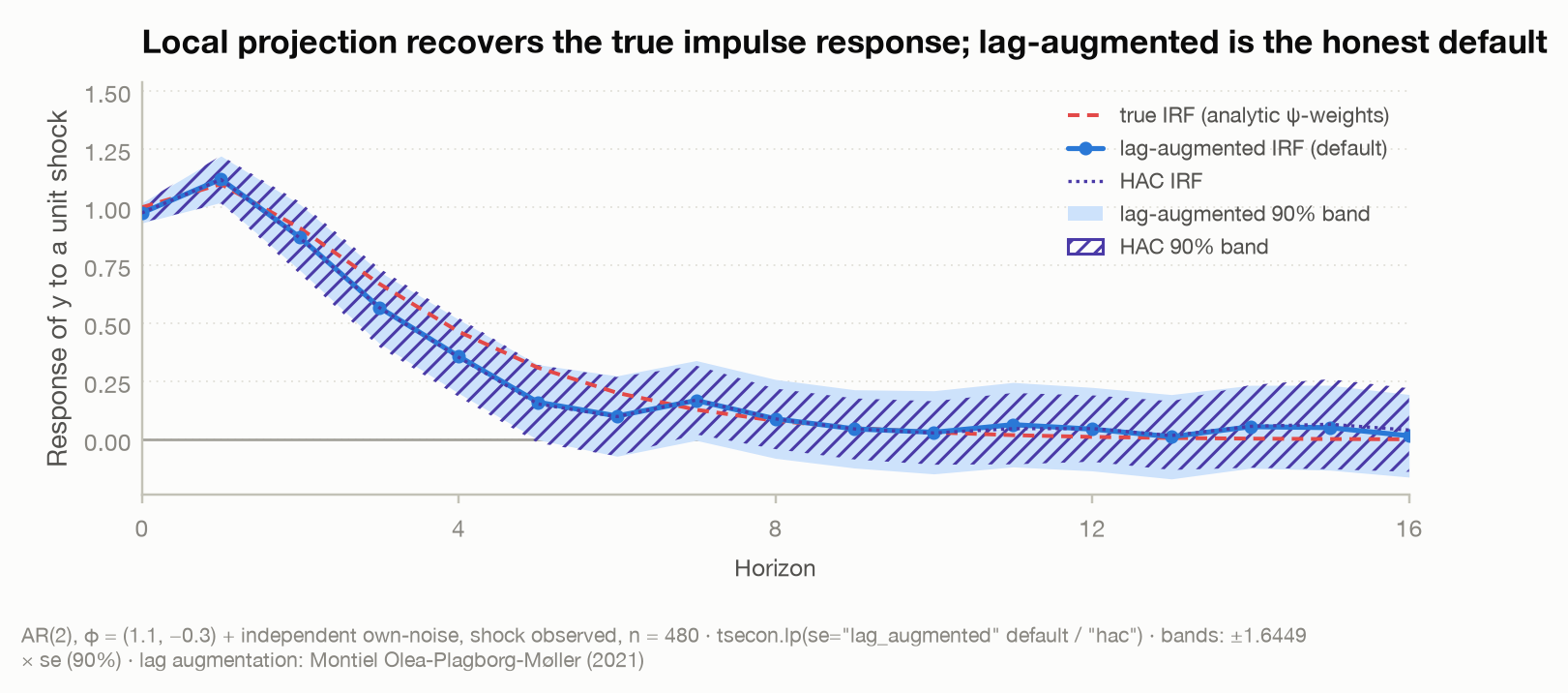
When it applies: you have a shock (or an instrument for one) and want its dynamic effect on one outcome, without committing to the cross-equation dynamics a VAR imposes. Local projections run one regression per horizon and read the IRF straight off the shock coefficient — robust to misspecified dynamics, and the modern default since Jordà (2005).
LP or VAR? They estimate the same impulse response (Plagborg-Møller & Wolf 2021); the choice is a bias-variance one, and it is measured rather than argued in chapter 16 — LP versus VAR, head to head: where the two finite-sample estimates coincide exactly, how bias, SD, RMSE and band coverage compare on a seeded Monte Carlo, and the rule this library recommends — fit both; take the lag-augmented LP as the point path and bands at horizons short relative to the sample; overlay a generously lagged VAR for the long horizons, where the LP's variance is the binding cost; and read a divergence between the two as a lag-length diagnostic, not a verdict.
d = json.load(open("fixtures/lp.json"))
y, shock, instrument = np.array(d["y"]), np.array(d["x"]), np.array(d["z"])

r = tsecon.lp(y, shock, horizons=16)              # se="lag_augmented" default (Montiel Olea–Plagborg-Møller)
r["irf"], r["se"]                                 # 90% band: irf ± 1.6449·se
Then branch by what you have:
- The shock is endogenous but you have an instrument — use per-horizon 2SLS, which also returns a first-stage effective F so you can spot a weak instrument:
iv = tsecon.lp_iv(y, shock, instrument, horizons=16, n_lag_controls=4)
iv["first_stage_f"]                             # first-stage strength
- You want a fiscal (integral) multiplier — cumulated response per
cumulated dollar of the impulse. This has its own entry point, because
lp_iv(..., cumulative=True)cumulates only the outcome (a cumulative IRF — a fine object, but not a multiplier; on the Ramey-Zubairy data it runs 7 to 49 where the true multiplier is ~0.7):
m = tsecon.lp_multiplier(y, shock, instrument, horizons=16)
m["multiplier"], m["se"], m["first_stage_f"]    # the Ramey-Zubairy integral multiplier
- The response differs by regime (recession vs expansion) — interact with a predetermined state indicator for one IRF per regime:
state = (np.arange(len(y)) % 2 == 0).astype(float)     # your 0/1 regime, known at t-1
st = tsecon.lp_state(y, shock, state, horizons=16, n_lag_controls=4)
st["irf_state1"], st["irf_state0"]              # per-regime responses
-
You have a panel of units all hit by the same shock — pool them; see section 5 (
panel_lp). -
The horizon-by-horizon IRF is jagged (short sample, noisy shock) — shrink it toward a smooth curve with
smooth_lp, a penalized B-spline in the horizon estimated jointly across horizons (Barnichon-Brownlees 2019).lam=0.0reproduces the raw per-horizon LP;lam="cv"picks the penalty by block cross-validation:
sm = tsecon.smooth_lp(y, shock, horizons=16, n_lag_controls=4, lam="cv")
sm["irf"], sm["se"], sm["lambda_used"]          # irf_raw / se_raw = the unsmoothed LP for comparison
Escape hatch — the response itself is nonlinear (thresholds, regime switching in the system, not just a known indicator): the generalized impulse response averages over histories and shock signs. See chapter 13 — the generalized impulse response.
Go deeper: chapter 9 — one regression per horizon, inference done right, LP-IV and multipliers · gallery figure
2d · …the shock is a whole curve, not a scalar¶
When it applies: the thing that moves is an entire function — the whole yield
curve shifts and twists, a cross-sectional distribution slides — and you want the
response of an outcome to a named scenario for that curve (a parallel shift, a
steepening). Compress the curve panel to a few functional principal components
(functional_pca, Inoue-Rossi 2021), then project the outcome on the scores.
import json, numpy as np, tsecon

t = json.load(open("fixtures/termstructure.json"))
curves = np.array(t["yields_panel"])              # T × M: one whole curve per period
y = curves.mean(axis=1)                            # an outcome driven by the curve (use your own series)
delta = np.ones(curves.shape[1])                   # the scenario: a parallel +1 shift across maturities

fp  = tsecon.functional_pca(curves, n_factors=3)   # eigenfunctions + scores; read fp["explained"]
fls = tsecon.flp_scenario(y, curves, delta, n_factors=3, horizons=8, n_lag_controls=2)
fls["response"], fls["se"]                         # single-equation (LP) IRF to the whole-curve shock
fvs = tsecon.fvar_scenario(y, curves, delta, n_factors=3, lags=2, horizon=8)
fvs["response_outcome"]                            # the VAR-form counterpart
Use flp_scenario for the local-projection reading (robust to misspecified
dynamics) and fvar_scenario for the VAR-form reading, and always report the
FPCA explained so the reader knows how much of the curve your factors capture.
This is frontier, tsecon-native territory with no off-the-shelf R/Stata
equivalent — treat the responses as exploratory, not settled.
Go deeper: chapter 15 — the term-structure frontier
2e · …I can defend a long-run, variance-share, instrument, or variance-regime restriction¶
When it applies: you want a point identification (one impact matrix, not a
set) and you have exactly one of five kinds of leverage. Each is a
different assumption — pick the one you can actually defend, and read the full
anatomy in the
structural-identification card.
All five take the reduced-form data matrix and are deterministic (no RNG). Below,
data is the 3-variable macro matrix from 2a.
- A long-run neutrality — some shock has no permanent effect on some variable (demand is neutral for output in the long run). Blanchard-Quah:
bq = tsecon.long_run_svar(data, lags=4, horizon=20)   # e.g. data = [dlog output, unemployment]
bq["cumulative_irf"]        # plot this for differenced variables; the neutral shock's level effect decays to 0
Check the VAR's roots first — the scheme is fragile near a unit root (Faust-Leeper).
For confidence bands use long_run_svar_bands (a bootstrap that re-identifies in
every draw, or the delta method). Read its card's per-cell coverage table first:
no arm covers every cell.
- A variance objective — you want the single shock that explains the most of a target's forecast-error variance over a business-cycle window (the "main business cycle" or technology/news shock):
ms = tsecon.max_share_svar(data, target=0, h0=6, h1=32, horizon=40)
ms["share_window"], ms["impact"]     # exclude_impact=True gives the Barsky-Sims news shock
- A measured instrument — a narrative surprise or high-frequency series that is relevant for one shock and exogenous to the rest (the modern monetary/tax default):
proxy = data[:, 2] + np.random.default_rng(0).standard_normal(len(data))  # use your real instrument
pr = tsecon.proxy_svar(data, proxy, norm_var=2, unit=1.0)   # proxy aligns to rows; NaN outside its window is dropped
pr["first_stage_f"], pr["irf"]       # check F first; bands via proxy_svar_bands, weak-IV sets via proxy_ar_sets
- Documented variance regimes — B is constant but the shock variances differ across known windows (crisis vs calm, announcement vs control days):
regime_labels = (np.arange(len(data)) >= len(data) // 2).astype(int)   # your documented split (two labels)
het = tsecon.hetero_svar(data, regime_labels)
het["B"], het["min_ratio_gap"]       # identified iff the variance ratios are distinct; the shocks carry no labels
- Non-Gaussian shocks and no restriction to spend — you distrust every economic story (no ordering, no instrument, no regime), but the shocks are plausibly independent and non-Gaussian (fat-tailed, skewed). Let the shape of the distribution identify B via independent-component analysis:
ng = tsecon.nongaussian_svar(data, lags=2, horizon=12)
ng["impact"], ng["shock_kurtosis"]   # FAILS under Gaussianity: kurtosis near 0 flags a weakly identified column
It point-identifies the whole B with no restriction — but fails if the shocks
are Gaussian (the diagnostic is shock_kurtosis), and column sign/order are
conventions.
The order of preference when more than one applies: if you have a credible
instrument, use it (proxy_svar makes the weakest assumptions about the rest of
the system); otherwise let the question choose — permanent-vs-transitory →
long_run_svar, "the dominant driver" → max_share_svar, documented volatility
shifts → hetero_svar, and — when you can spend no economic restriction but the
shocks are non-Gaussian — nongaussian_svar.
Escape hatch — short sample, and you don't want to hand-tune shrinkage. All of these estimate a reduced-form VAR first, and on short macro samples that VAR is noisy. A hierarchical BVAR lets the data pick the Minnesota tightness by maximizing the marginal likelihood, rather than the folklore 0.2:
hb = tsecon.bvar_hierarchical(data, lags=2, optimize="lambda1")
hb["lambda1_opt"], hb["log_marginal_likelihood"]   # the data's tightness vs hb["lambda1_fixed_log_ml"]
See section 2a for the Bayesian IRF-band route and chapter 10.
Go deeper: chapter 8 — long-run, max-share, proxy, and heteroskedasticity identification · structural-identification model card
2f · …and now I want to decompose, narrate, or prior-robustify the shock¶
When it applies: you have already identified a shock (by any scheme above)
and want the standard follow-up objects — a variance decomposition, a historical
attribution, one coherent IRF instead of a median that mixes models, honest
prior-robust bounds, or a set sharpened with episode knowledge. These five tools
take an identification; they do not invent one. Reusing the data matrix and
sign restrictions from 2b:
- A variance decomposition for the identified shock —
var_fevdonly knows the recursive Cholesky; feed any impact matrixA0(here the coherent Fry-Pagan draw's) tostructural_fevd:
fp = tsecon.fry_pagan_svar(data, restr, lags=2, horizon=16, n_draws=500, seed=1)
A0 = np.asarray(fp["median_target_irf"])[0]                # a valid identified impact matrix
sf = tsecon.structural_fevd(data, lags=2, horizon=16, impact=A0)
np.asarray(sf["fevd"])[8, 0, 0]        # 0.604: demand-shock share of GDP's h=8 FE variance; each row sums to 1
- One coherent model, not the median band — the pointwise median mixes
mutually inconsistent draws.
fry_pagan_svarreturns the single accepted draw closest to it (a companion to the band, not a replacement):
mt  = np.asarray(fp["median_target_irf"])   # coherent [h][var][shock]; mt[0] is an A0
med = np.asarray(fp["median_irf"])          # the incoherent pointwise median
mt[0, 0, 0], med[0, 0, 0]              # (0.702, 0.560): the coherent impact response is not the median
- How much did shock j drive variable i in episode X — the historical
decomposition, with an exact adding-up identity
y = baseline + Σ_j hd:
hd = tsecon.historical_decomposition(data, lags=2, identification="cholesky")
hd["hd"]          # [time][variable][shock] contributions; identification="sign" gives the weighted set
hd["baseline"]    # deterministic + initial-condition path; times are 0-based effective-sample indices
- Prior-robust bounds — the Haar rotation prior never washes out, so part of
a sign-restricted band is artifact.
robust_svar_boundsreports the exact identified set with that prior removed (Giacomini-Kitagawa):
rb = tsecon.robust_svar_bounds(data, restr, lags=2, horizon=16, n_draws=500, seed=1, alpha=0.10)
rb["robust_ci_lower"][0][0][0], rb["robust_ci_upper"][0][0][0]   # (0.000, 0.833): wider than the sign band's (0.119, 0.756)
rb["restricted_shocks"]         # [0] — unrestricted shocks are NaN; empty_set_rate is a GK diagnostic
- Shrink the set with episode knowledge — if the historical record tells you a
shock's sign or that it dominated an episode,
narrative_svarimposes it by importance-reweighting (Antolín-Díaz-Rubio-Ramírez):
narr = [{"type": "contribution", "variable": 0, "shock": 0, "start": 73, "end": 75, "rule": "most"}]
nv = tsecon.narrative_svar(data, restr, narr, lags=2, horizon=16, n_draws=500, seed=1, n_weight_draws=200)
nv["weights"], nv["diagnostics"]["ess"]   # per-draw weights (mean 1) and the effective sample size — watch it
With narrative_restrictions=None it is sign_restricted_svar, bit-for-bit,
so it is a safe default. A collapsing ess means the narrative is fighting the
posterior — the diagnostic to read.
The rule of thumb: report structural_fevd and historical_decomposition
alongside any IRF; add fry_pagan_svar for a single coherent set of numbers;
and for a set-identified result headed for publication, show
robust_svar_bounds next to the sign band so the reader sees how much was prior
rather than data — with narrative_svar when you can defend an episode.
Go deeper: chapter 8 — sign restrictions, honest bands, and the two critiques · post-identification tools in the model card
3 · I have quarterly GDP and monthly indicators¶
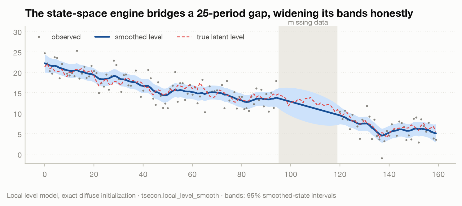
The question in plain words: your target arrives late and infrequently (quarterly GDP), but related indicators arrive often and early (monthly surveys, weekly claims, daily financial conditions). You want a current-quarter estimate that updates as data land — a nowcast — despite the frequency mismatch and the ragged edge where the newest series run ahead of the oldest.
The decision path turns on how many high-frequency series and how ragged the edge:
- Many indicators, genuine ragged edge → a dynamic factor model. It extracts a few common factors by a Kalman filter that handles missing values at the edge natively, then maps the edge factor to the target. This is the central-bank workhorse.
import json, numpy as np, tsecon

panel = np.array(json.load(open("fixtures/tsecon-nowcast.json"))["panel"])   # T x N
panel[-1, 4:] = np.nan                                     # the ragged edge: newest month partial

nc = tsecon.dfm_nowcast(panel, n_factors=1)
nc["nowcast"]                                              # current-period estimate
nc["edge_factor"]                                          # the factor at the ragged edge
- One (or few) indicators, and you want an explicit lag polynomial → a MIDAS regression. Whether to restrict the lag weights depends on the frequency ratio:
m = json.load(open("fixtures/midas.json"))
y = np.array(m["y"])                        # low-frequency target
X = np.array(m["X_stacked"]).T              # nobs × K, columns = HF lags, most-recent first

u = tsecon.umidas(y, X, se_type="hac")                    # unrestricted: one OLS coef per lag
w = tsecon.weighted_midas(y, X, scheme="beta")            # restricted: a smooth weight curve
w["weights"], w["converged"]                              # weights sum to 1; always check convergence
Use umidas when the ratio is small (monthly→quarterly, K≈3): with few
lags, plain OLS beats the restriction. Switch to weighted_midas
(scheme="exp_almon" or "beta") when the ratio is large (daily→quarterly),
where an unrestricted regression would have dozens of coefficients and no hope
of estimating them — the smooth curve is what makes it feasible.
Escape hatch — "why did my nowcast move this morning?" After a new data vintage lands, decompose the revision into per-datapoint news contributions (here two vintages differ only at the ragged edge, so the revision is news):
old_vintage = panel.copy(); old_vintage[-1, :] = np.nan; old_vintage[-2, 3:] = np.nan
new_vintage = panel.copy(); new_vintage[-1, :4] = np.nan       # newer data have arrived

nw = tsecon.dfm_news(old_vintage, new_vintage, target_series=0, n_factors=1)
nw["total_revision"], nw["contributions"]      # which release moved the number
See chapter 11 — news decomposition.
Go deeper: chapter 11 — the two-step DFM nowcast, MIDAS, weighted_midas vs umidas · gallery figure (the shared Kalman engine)
4 · My volatility has fat tails or jumps¶
The question in plain words: the size of movements is what you care about (risk, options, margins), and your returns are not tidy Gaussian noise — they have heavy tails and the occasional isolated jump that a naive filter would mistake for a lasting change in volatility.
The decision path turns on what data you hold:
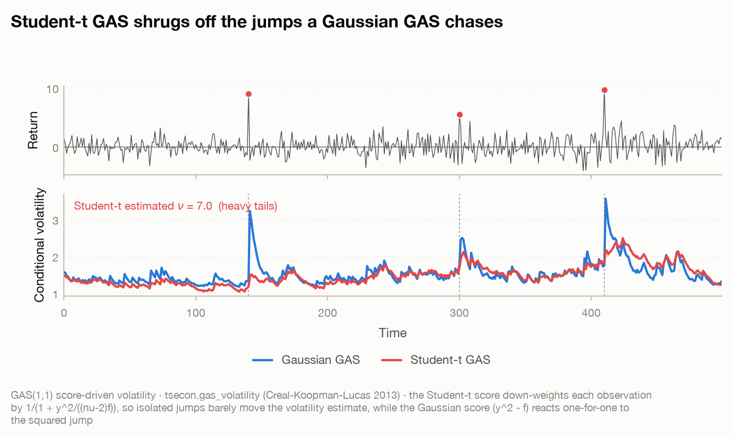
- A daily return series with fat tails / jumps → a score-driven (GAS) volatility model with a Student-t density. Its update is driven by the score of the observation density, which automatically down-weights a jump as a tail draw instead of over-reacting to it:
import json, numpy as np, tsecon

returns = np.array(json.load(open("fixtures/realized.json"))["measures_small"]["returns"])

st = tsecon.gas_volatility(returns, density="student_t")   # estimates the dof nu
st["nu"], np.sqrt(st["variance"])                          # low nu ⇒ heavy tails; the filtered vol path
Compare density="gaussian" to see the robustness: the Gaussian filter
spikes at each jump, the Student-t barely moves.
- Intraday (high-frequency) returns within a day → realized measures split the day's variation into a continuous part and a jump part, model-free:
rm = tsecon.realized_measures(returns)         # {'rv', 'bipower', 'jump'}
jt = tsecon.bns_jump_test(returns)             # Barndorff-Nielsen–Shephard jump test
- A series of daily realized variances and you want to forecast it → the HAR-RV regression (daily/weekly/monthly components) is the standard, cheap, hard-to-beat benchmark:
rv = np.array(json.load(open("fixtures/realized.json"))["rv_series"])
hr = tsecon.har_rv(rv, variant="log")          # "level", "log", or "sqrt"; HAC SEs
hr["params"], hr["rsquared"]
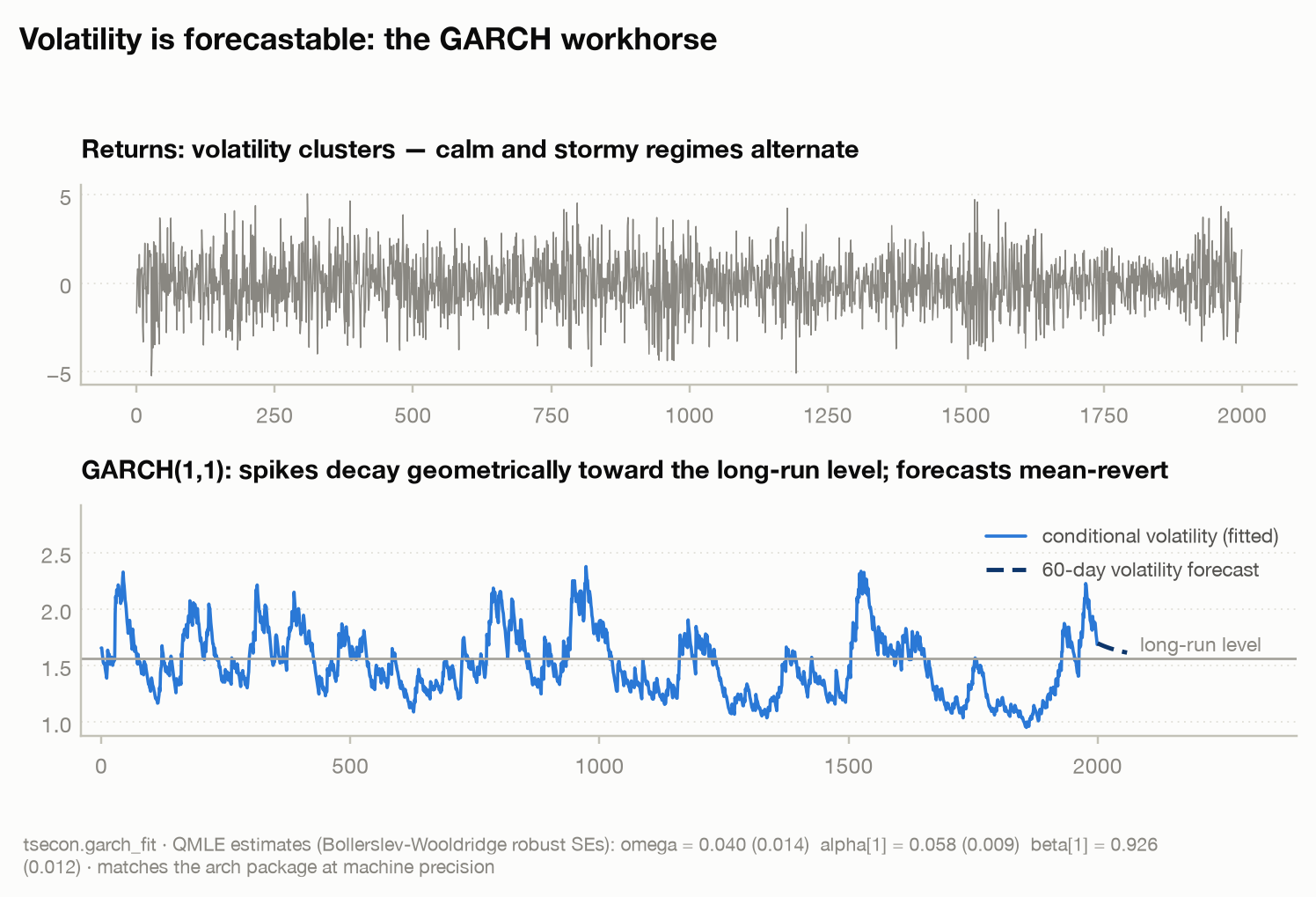
Escape hatch — plain volatility clustering, no jumps. If the tails are mild
and you just want the classic conditional-variance model on a daily return
series — with robust standard errors and a multi-step forecast fan — use
garch_fit (and vol="gjr" for the leverage/asymmetry effect, dist="t" for
fat tails):
daily = np.array(json.load(open("fixtures/garch.json"))["returns"])   # a daily return series
g = tsecon.garch_fit(daily, vol="garch", dist="t", forecast_horizon=60)
g["conditional_volatility"], g["variance_forecast"]                   # fitted path + forecast fan
See chapter 6 — GARCH(1,1) and
its gallery figure. For a portfolio of assets,
ccc_garch / dcc_garch give the correlation dynamics.
Escape hatch — the downside risk of an outcome, not its variance.
Volatility is symmetric; sometimes the question is one-tailed ("how bad is the
5th-percentile GDP outcome a year out, given today's financial conditions?").
That is a conditional quantile, not a conditional variance. growth_at_risk
fits the Adrian-Boyarchenko-Giannone (2019) conditional-quantile Growth-at-Risk
directly — the lower tail of the h-ahead outcome given conditioning variables:
rng = np.random.default_rng(1); T = 200
fci = rng.standard_normal(T)                                  # a financial-conditions index
g   = 0.3 - 0.8 * fci + rng.standard_normal(T) * (1 + 0.5 * np.abs(fci))
gar = tsecon.growth_at_risk(g, fci.reshape(-1, 1), horizon=4, taus=[0.05, 0.5, 0.95])
gar["current"]                                                # [5%, 50%, 95%] read for today; [0] is GaR
For the dynamic version — the impulse response at a quantile rather than the
mean path — quantile_lp(y, shock, taus=..., horizons=...) runs a quantile
local projection per horizon; quantile_regression(y, X, taus=...) is the static
building block (the check-loss analogue of ols).
Go deeper: chapter 6 — score-driven volatility, realized measures, HAR · gallery figure
5 · I have a panel with heterogeneous units¶
The question in plain words: you have many units (countries, firms, banks) observed over time, and you suspect they do not all share the same slope or the same dynamics. Pooling them into one regression is not merely inefficient here — if the coefficients truly differ, it is inconsistent. The right estimator depends on what kind of heterogeneity you allow and whether a common factor contaminates the regressors.
The decision path:
| Your situation | Reach for |
|---|---|
| One common slope; confounders are unit-fixed; want robust SEs | panel_fe (se_type="cluster" or "driscoll_kraay") |
| One common slope, but a regressor of interest is time-invariant | panel_re (random effects) — valid only if the unit effect is uncorrelated with the regressors |
| FE or RE? | the Mundlak check: add the unit means of the time-varying regressors to panel_re; its slopes then equal panel_fe's, and a cluster Wald on the means (from the returned cov) is the robust Hausman test — reject → panel_fe |
| FE or FD? | panel_fd when the errors look more like a random walk than white noise (FE when serially uncorrelated); both remove the unit effect; at T = 2 they coincide. constant=True matches plm / Stata D.y D.x |
| Cross-sectional pricing: one regression per period, averaged | panel_fama_macbeth — right for a time effect, wrong for a persistent firm effect (its SE then covers far below nominal; cluster by entity instead) |
| Slopes differ across units; no common factor | panel_mean_group(method="mg") |
Slopes differ and an unobserved common factor drives y and x |
panel_mean_group(method="cce") |
| A long-run relationship you want to pool, with unit-specific short-run dynamics | panel_pmg |
| Each unit has its own multivariate dynamics (its own VAR) | mean_group_var |
| A single shock felt by all units; want its pooled IRF | panel_lp |
The heterogeneous estimators take lists of per-unit arrays (response
vectors ys, regressor matrices xs, each T_i × k):
import json, numpy as np, tsecon

d = json.load(open("fixtures/tsecon-panelts.json"))
yP, xP = np.array(d["y"]), np.array(d["x"])                 # yP: N×T,  xP: k×N×T
N = yP.shape[0]
ys = [yP[i] for i in range(N)]
xs = [xP[:, i, :].T for i in range(N)]                      # each T×k

mg  = tsecon.panel_mean_group(ys, xs, method="mg")          # average of per-unit OLS slopes
cce = tsecon.panel_mean_group(ys, xs, method="cce")         # + cross-section averages purge the factor
pmg = tsecon.panel_pmg(ys, xs)                              # pooled long-run θ, unit-specific EC speed
mg["coef"], mg["se"], cce["coef"], pmg["theta"], pmg["phi_bar"]
For a common-shock impulse response (the panel analogue of local
projections) and per-entity VARs, the layouts differ — panel_lp takes the
N × T outcome and a length-T shock; mean_group_var takes a list of
per-entity T_i × k matrices:
p = json.load(open("fixtures/panel.json"))["panel"]
outcome, shk = np.array(p["y"]), np.array(p["shock"])       # N×T outcome, length-T common shock
plp = tsecon.panel_lp(outcome, shk, horizon=6, n_lag_controls=2, se_type="driscoll_kraay")
plp["irf"], plp["se"], plp["nobs"]                          # watch nobs fall across horizons

sys = np.array(json.load(open("fixtures/var.json"))["data_100dlog_gdp_cons_inv"])   # a T×k system
entities = [sys[:120, :], sys[80:, :]]                      # list of per-entity T_i×k systems
mgv = tsecon.mean_group_var(entities, lags=1, trend="c", horizon=6, response=0, impulse=0)
mgv["irf_path"]                                             # averaged orthogonalized IRF
Escape hatch — few units (< ~30). Clustered asymptotics are unreliable with
few clusters; the point estimate from panel_fe still stands, but treat its
standard errors with caution and prefer a wild cluster bootstrap. For a long
panel LP in a short panel, correct the Nickell bias that grows like O(h/T):
panel_lp(..., bias_correction="spj") (Mei-Sheng-Shi split-panel jackknife —
corrects the points and recomputes the standard errors) or
panel_lp(..., jackknife=True) (Dhaene-Jochmans — points only, plug-in SEs;
see the panel model card for the measured difference).
Escape hatch — is the panel even stationary? Before a panel VAR or a
cointegration analysis, test the joint null "every unit has a unit root" —
the panel analogue of section 1.
panel_unit_root runs the three first-generation classics: "ips"
(Im-Pesaran-Shin, heterogeneous alternative, the default), "fisher"
(Maddala-Wu/Choi p-value combination), and "llc" (Levin-Lin-Chu, a common
root, balanced panels only). Pooling across units buys far more power than any
single-series ADF.
r = tsecon.panel_unit_root(outcome, test="ips", regression="c")   # outcome is N×T
r["statistic"], r["p_value"]          # small p ⇒ reject the joint unit-root null
r["per_unit_pvalue"]                  # which units drive the verdict
These are first-generation tests: they assume cross-sectional independence and distort in size when a common factor correlates the units (the second-generation CIPS/PANIC tests under cross-sectional dependence are on the roadmap). Run Pesaran's CD check first if a global factor is plausible.
Go deeper: chapter 14 — fixed effects, panel unit roots, mean-group VAR, the CCE cure, panel LP
6 · My regressor is highly persistent¶
The question in plain words: you are running a predictive regression — next period's return on a valuation ratio, say — and the predictor is nearly a unit root (dividend yield, interest-rate spreads). Standard t-statistics over-reject wildly here: the Stambaugh bias and the near-integrated regressor break the textbook asymptotics, and you will "find" predictability that is not there.
The honest routing. The dedicated fix ships today:
tsecon.predictive_regression(r, x) returns three views of the same regression
in one call — plain OLS (the misleading benchmark), the Stambaugh (1999)
finite-sample bias correction, and the IVX estimator with a persistence-robust
Wald test (Kostakis, Magdalinos & Stamatogiannis 2015) that keeps its size
whether the predictor is stationary, near-integrated, or an exact unit root. For
several persistent predictors at once, tsecon.ivx_test(r, xs) gives the joint
IVX test — solid at a few predictors, but its size grows with k at the default
tuning (measured 0.28 at k=8, ρ=1, nominal 5%, and larger samples do not fix it),
so pass joint="bonferroni" for a many-predictor joint test (measured size at
or below nominal at every k; alpha=0.5 is the weaker mitigation) and see the
measured size caveat.
Read the IVX Wald verdict as your headline; use Stambaugh for a debiased
point estimate; keep OLS only to show what the correction bought you. See the
predictive-regressions model card.
Do not reach for a naive OLS t-statistic instead.
A complementary route. If your persistent predictor is also instrumentable,
you can additionally cast the regression as IV and use HAC-robust GMM
(iv_gmm) — this side-steps part of the endogeneity that drives the Stambaugh
bias, though predictive_regression's IVX view is the direct near-unit-root fix. It is
section 10's estimator (X holds the
endogenous predictor, Z its instruments) with a HAC weight for the serially
correlated moments:
import json, numpy as np, tsecon

g = json.load(open("fixtures/gmm.json"))
y = np.array(g["y"]); const = np.ones(len(y))
X = np.column_stack([const, g["w"], g["x"]])          # x: the persistent/endogenous regressor
Z = np.column_stack([const, g["w"], g["z1"], g["z2"]])   # instruments include the exogenous columns

fit = tsecon.iv_gmm(X, Z, y, method="2step", weight="hac")   # HAC weight for serial correlation
At minimum, always pair the estimate with an honest out-of-sample test
(backtest + dm_test, chapter 5) against the
historical-mean benchmark, and report unit-root diagnostics on the predictor
(section 1) so the reader
can judge how near-integrated it is. In-sample predictive significance on a
persistent regressor should be treated as a hypothesis, not a finding, until it
survives the IVX verdict and an out-of-sample test.
Go deeper: ROADMAP.md §10 (extension E3) · chapter 10 — endogenous IV via GMM
7 · I have many candidate predictors¶
The question in plain words: you have far more plausible predictors than you can estimate reliably — dozens of indicators, most of them noise — and OLS will overfit. You want the procedure itself to select, and you want to tune it without letting the future leak into the past.
The decision path turns on whether you want selection (a sparse model) or just shrinkage (a dense, stabilized one):
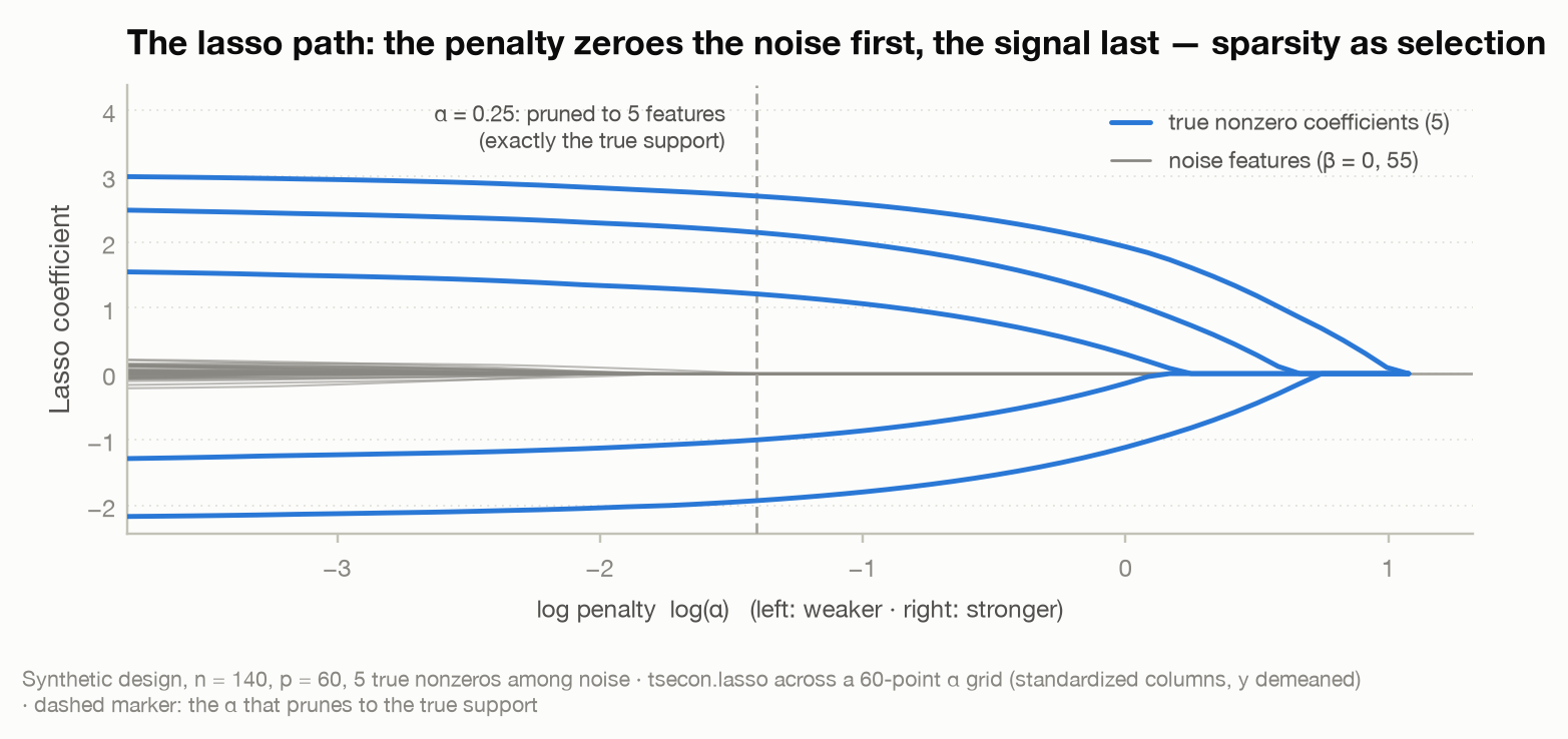
- Sparse selection — the LASSO zeros out most coefficients. For better selection consistency use the adaptive LASSO (re-weighted penalty, the oracle property); to pick the penalty by information criterion, sweep the whole path:
import json, numpy as np, tsecon

m = json.load(open("fixtures/ml.json"))
X, y = np.array(m["X_standardized"]), np.array(m["y_centered"])

al   = tsecon.adaptive_lasso(X, y, alpha=0.05)      # oracle-weighted L1
path = tsecon.lasso_path(X, y)                      # full path + AIC/BIC selection
path["bic_best"], path["lambdas"], path["coefs"]    # coefs at the BIC-optimal lambda
- Tune honestly — never use plain k-fold on time series; it trains on the future. Use leakage-safe splits with an embargo/purge, then loop your CV over them:
splits = tsecon.cv_splits(200, scheme="expanding", train=100, horizon=1, step=20)
for s in splits:                                    # each s = {"train": [...], "test": [...]}
    X[s["train"]], X[s["test"]]                     # fit on train, score on test — no overlap
Escape hatch — shrink, don't select. If the predictors are correlated and
you believe all of them matter a little, sparsity is the wrong prior: use
ridge (shrinks, never zeros) or elastic_net (the in-between). If a handful
of latent factors drive the whole cross-section, extract them first with
factor_model (Bai-Ng picks the number) and predict on the factors — the
diffusion-index approach.
Go deeper: chapter 12 — shrinkage with a frequentist face, leakage comes first, the landed functions · gallery figure
8 · I need spillovers across markets¶
The question in plain words: you have many markets or institutions and you want to know who transmits shocks to whom, and how connected the system is as a whole — a directed, time-varying map of spillovers, not just a correlation matrix.
The decision path. The Diebold-Yilmaz framework reads spillovers off a VAR's generalized forecast-error variance decomposition (order-invariant, so you avoid the Cholesky-ordering argument). One call returns the total index and the directional pieces:
import json, numpy as np, tsecon

c = json.load(open("fixtures/connect.json"))
data = np.array(c["data"])
if data.shape[0] < data.shape[1]:                   # ensure T × k (time down the rows)
    data = data.T

cn = tsecon.connectedness(data, lags=2, horizon=10)
cn["total"]                                         # system-wide connectedness (percent)
cn["to_others"], cn["from_others"], cn["net"]       # directional spillovers per market
cn["pairwise_net"]                                  # who-shocks-whom matrix
Read net to find net transmitters (positive) versus receivers (negative), and
roll the window to watch connectedness spike in crises — the headline use of
the measure.
Escape hatch — the markets share a common stochastic trend. If the series
are cointegrated (I(1) but tied together in the long run), model the shared
trend explicitly rather than the spillovers of their differences: test with
johansen and estimate the error-correction system with vecm. For a single
candidate relationship — one dependent series regressed on the others — the
lighter phillips_ouliaris residual test asks the yes/no question directly
(null: no cointegration), the semiparametric Engle-Granger route; reach for
johansen when you need the number of cointegrating vectors in a larger system.
When you cannot say whether the regressors are I(0) or I(1) — the case unit-root
pre-tests handle worst — ardl_bounds_test(y, x) runs the Pesaran-Shin-Smith
bounds test: a level relationship when p_value_upper is small whatever the
regressors are, none when p_value_lower is large, inconclusive in between; read
its t_statistic on the lagged level too, since a rejecting F with a near-zero t
is the degenerate case the F alone hides.
po = tsecon.phillips_ouliaris(data[:, 0], data[:, 1:], trend="c")   # y on the other columns; no constant column
po["stat"], po["pvalue"]                                             # small p ⇒ reject "no cointegration"
See
chapter 7 — cointegration.
If instead one policy variable and hundreds of indicators are in play,
favar compresses the indicators to factors and traces one policy shock across
all of them (chapter 7 — FAVAR).
Go deeper: chapter 7 — connectedness (Diebold-Yilmaz)
9 · I want to fit a yield curve¶
The question in plain words: you have a dozen bond yields at different maturities that move almost in lockstep, and you want to compress them to a few interpretable numbers — level, slope, curvature — to store, interpolate, or forecast the curve.
The decision path turns on whether you have one curve or a panel, and whether the curve has a second bend:
- One curve, summarize or interpolate → Nelson-Siegel: three factors, a single OLS at a fixed decay, no optimizer. The field standard.
import json, numpy as np, tsecon

t = json.load(open("fixtures/termstructure.json"))
maturities, yields = np.array(t["maturities"]), np.array(t["yields_date100"])

ns = tsecon.nelson_siegel(maturities, yields, decay=0.0609)   # or optimal_lambda=True to fit the decay
ns["level"], ns["slope"], ns["curvature"], ns["rsquared"]
- The curve has a genuine second hump (long maturities, unusual regimes) → Svensson adds a fourth factor. Use it only when you see systematic Nelson-Siegel residuals at the far end; otherwise the two decays fight over the same feature and the fit blows up.
sv = tsecon.svensson(maturities, yields, lambda1=0.0609, lambda2=0.03)
sv["rsquared"]        # compare to ns["rsquared"]: a rounding-error gain ⇒ don't bother
- A panel of curves you want to forecast → dynamic Nelson-Siegel fits the three factors every period and models the factor series as AR(1)s, collapsing a many-maturity forecast to three:
panel = np.array(t["yields_panel"])                  # T × n_maturities
dns = tsecon.dynamic_ns(panel, maturities, decay=0.0609)
dns["forecast"]["yields"]                            # next-period curve, all maturities
dns["forecast"]["ar1_phi"]                           # factor persistences — the forecast engine
Escape hatch — pricing, or the zero lower bound. Nelson-Siegel is a
statistical fit; it does not forbid arbitrage. For derivative pricing you want
an arbitrage-free model: tsecon.afns_adjustment adds the Christensen-Diebold-
Rudebusch (2011) closed-form yield-adjustment term to a Nelson-Siegel curve to
make it arbitrage-free (see the AFNS model card).
When yields sit near zero you want a shadow-rate model, still on the roadmap
(chapter 15 — the frontier).
Always settle whether a DNS forecast beats a random walk with a proper
backtest (chapter 5) before trusting it.
Go deeper: chapter 15 — Nelson-Siegel, Svensson, dynamic Nelson-Siegel
10 · Endogenous regressor + instruments¶
The question in plain words: a regressor is correlated with the error — simultaneity, measurement error, an omitted driver — so OLS is biased, but you have instruments that move the regressor without touching the error directly. You want a consistent estimate and a test of whether your instruments are credible.
The decision path turns on whether the moment conditions are linear in the parameters:
- Linear IV (the common case) →
iv_gmm. Stack the exogenous regressors into bothXand the instrument matrixZ; put the endogenous regressor inXand its excluded instruments inZ. When over-identified, it returns Hansen's J test of the over-identifying restrictions for free.
import json, numpy as np, tsecon

g = json.load(open("fixtures/gmm.json"))
y, x, w = np.array(g["y"]), np.array(g["x"]), np.array(g["w"])
z1, z2  = np.array(g["z1"]), np.array(g["z2"])
const = np.ones(len(y))

X = np.column_stack([const, w, x])          # x is endogenous; const, w exogenous
Z = np.column_stack([const, w, z1, z2])     # instruments INCLUDE the exogenous columns

fit = tsecon.iv_gmm(X, Z, y, method="2step", weight="robust")
fit["params"], fit["bse"]                   # robust sandwich SEs
fit["j_stat"], fit["j_pval"]                # Hansen J: is any instrument invalid?
Choose method: "2sls" when just-identified or errors are homoskedastic;
"2step"/"iterated" when over-identified and errors are
heteroskedastic/serially correlated (there GMM beats 2SLS and only GMM gives
the J test). Pass weight="hac" for serially correlated moments — the rule,
not the exception, in macro time series.
- Nonlinear moments (Euler equations, structural systems, nonlinear-in-
parameters IV) →
gmm_nonlinear. Supply a Python callback returning then × mmatrix of per-observation moment contributions; the library minimizes the GMM objective by Nelder-Mead.
rng = np.random.default_rng(0)
data = rng.exponential(scale=0.5, size=2000)          # true rate lambda = 2

def moments(theta):                                   # returns (n, 2): over-identified
    lam = theta[0]
    return np.column_stack([data - 1.0/lam, data**2 - 2.0/lam**2])

res = tsecon.gmm_nonlinear(moments, initial=[1.0])
res["params"], res["converged"], res["gbar"]          # always check converged and gbar ≈ 0
For the efficient estimator, do the standard two step: estimate once with
the identity weight, build S from the first-step moments, and re-optimize
with weight=np.linalg.inv(S).flatten().
Escape hatch. For linear IV always prefer iv_gmm over gmm_nonlinear: it
is a closed-form solve, and it returns sandwich SEs and the J test that the
simplex search does not. The LP-IV multipliers of
section 2c are exactly
iv_gmm(..., method="2sls") applied per horizon.
Go deeper: chapter 8 — linear IV-GMM, nonlinear GMM
When none of these fit¶
Three more entry points that do not have their own symptom above but come up often:
-
"My series switches between regimes on its own" (recession/expansion, high/low volatility, not a known indicator) →
markov_switching_arfits the regimes and their transition probabilities by EM; chapter 4 — regimes and thresholds and chapter 13. -
"I just need a solid univariate forecast" →
arima_fitfor the classical route,theta_forecastfor the competition-grade benchmark, wrapped inbacktestfor honest evaluation; chapter 5. -
"Is my model's forecast actually better than the benchmark?" → never claim it without a test:
dm_test(Diebold-Mariano),cw_test(nested models),gw_test(Giacomini-White unconditional, fixed rolling window — the conditional GW test is still a roadmap item); chapter 5 — the Diebold-Mariano test.
For the full method-by-method treatment with the math and the classic mistakes, every section above links into the 15-chapter guide; for worked, figure-rich examples on synthetic data, see the gallery.