Replication — Blanchard & Quah (1989)
The founding paper of long-run identification, and the first item the
roadmap's Phase-2 gate names. Blanchard and Quah (1989) put real output growth
and the unemployment rate in a bivariate VAR and separate two structural
disturbances with a single restriction that theory supplies without any stand
on within-quarter timing: demand disturbances have no permanent effect on
the level of output, so the supply disturbance is the only source of
output's stochastic trend. Their findings, read off their Figures 1–2 and
their variance-decomposition table: demand disturbances have a hump-shaped
effect on output that peaks after about a year and vanishes within a few
years; the effect on unemployment is, up to scale, a mirror image; the
effect of supply disturbances on output builds to a permanent plateau; a
favourable supply disturbance raises unemployment on impact; and demand
disturbances account for most of the forecast-error variance of output at
short horizons and of unemployment throughout. This page is the natural
flagship for
long_run_svar,
its confidence bands
long_run_svar_bands,
and historical_decomposition(identification="impact").
What this is, and is not. A design replication at figure-reading resolution, not a numerical one. The paper used real GNP and unemployment for 1948Q2–1987Q4; that vintage is not reachable from the build environment (FRED and the institutional archives refuse the request), and the bundled series is later-vintage real GDP over 1959–2009 — a different output measure, a different deflator base, and a sample that adds the Great Moderation and the 2008–09 recession while losing the 1950s. So the page reproduces the paper's design — the same transformations, lag order, restriction and objects — and pins the qualitative findings with stated numerical bands. It makes no claim of parity with the 1989 tables, and every assertion in the CI guard is a shape claim, never a published digit.
The data is the bundled statsmodels.datasets.macrodata — US real GDP
(billions of chained 2005 dollars) and the civilian unemployment rate,
quarterly 1959Q1–2009Q3, US-government statistics, public domain — committed
as a two-column extract at
fixtures/macrodata_bq.csv so the CI
guard runs offline like every other replication page (tsecon ships no data
loaders). --write-fixture regenerates the extract from the bundle, and the
guard checks equality with it whenever statsmodels is importable. The script
runs in about three seconds on the build machine, including two sets of 1,000
bootstrap replications (plain and Kilian-corrected), the delta-method bands and
three figures.
The identification
Output growth is 100·Δlog(real GDP), demeaned separately before and after
1974Q1 — Blanchard-Quah's own treatment of the post-1973 productivity
slowdown, and the part of the design everything hinges on (see the
sensitivity table below); the unemployment rate is linearly detrended, as
in the paper. The VAR carries a constant, so demeaning as such is inert — only
the break and the trend change anything. The lag order is the paper's
eight; on this sample the information criteria pick two (BIC, HQ) or
three (AIC), and the findings survive at those orders too (the CI guard
re-runs them). The VAR(8) is stable (smallest reciprocal-root modulus 1.153,
comfortably outside the unit circle — the Faust-Leeper fragility check the
model card asks for).
long_run_svar returns the impact matrix impact (B), the long-run matrix
long_run (C(1)·B, lower-triangular by construction), the structural
responses irf and their running sums cumulative_irf, and fevd. With the
paper's ordering (output growth first, unemployment second) the default
recursive long-run pattern is the Blanchard-Quah restriction. One
convention to be explicit about: tsecon signs each disturbance so the
long-run diagonal is positive, which labels the demand disturbance by its
cumulative effect on unemployment. Blanchard-Quah sign it as expansionary,
with output up on impact and unemployment down. That is
impact_signs=[(0, 1)], which anchors the demand column on output's impact
response and negates it here. It is a sign convention, not a different model,
and the variance shares are invariant to it. Before 0.11.0 the script
flipped the column by hand.
long-run matrix C(1)B            impact matrix B (one-s.d. disturbances)
  [[+0.480   0.000]                [[+0.243  +0.708]
   [+3.136  −5.890]]                [+0.137  −0.188]]
The upper-right zero is the imposed neutrality; the supply disturbance's permanent effect on output is +0.48 percent per one-standard-deviation disturbance.
The result
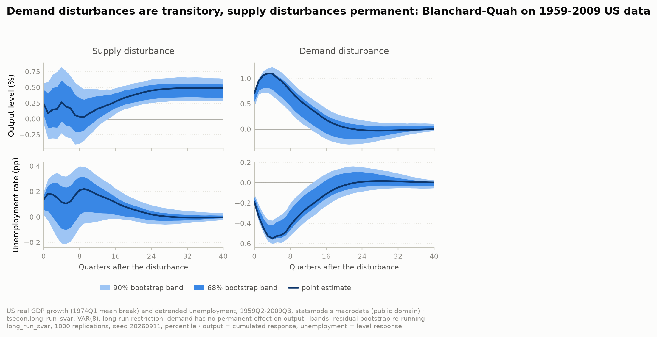
The objects the paper plots: output's cumulated response (the level) and
unemployment's plain response, in percent and percentage points per
one-standard-deviation disturbance, with 68% and 90% percentile bands from
long_run_svar_bands' residual bootstrap (below).
| response | h = 0 | h = 2 | h = 4 | h = 8 | h = 12 | h = 20 | h = 40 | extremum (h) |
|---|---|---|---|---|---|---|---|---|
| output ← supply | +0.243 | +0.147 | +0.264 | +0.031 | +0.161 | +0.378 | +0.486 | +0.490 (34) |
| output ← demand | +0.708 | +1.063 | +1.095 | +0.761 | +0.439 | +0.037 | −0.004 | +1.100 (3) |
| unemployment ← supply | +0.137 | +0.176 | +0.116 | +0.210 | +0.175 | +0.059 | −0.003 | +0.220 (9) |
| unemployment ← demand | −0.188 | −0.445 | −0.550 | −0.421 | −0.241 | −0.026 | +0.003 | −0.550 (4) |
The paper's findings, read at figure resolution — each with the band the CI
guard (test_replication_blanchard_quah.py)
pins it to:
- Demand → output is hump-shaped and transitory. Impact +0.708, peak +1.100 at h = 3 (the paper: "after about a year"), +0.037 at h = 20, −0.004 at h = 40 — zero at infinity by construction, and effectively zero after five years. Guard: peak at h ∈ [1, 8] and at least 0.1 above the impact; |h = 20| < 0.15; |h = 40| < 0.05 and below 10% of the peak.
- Supply → output is permanent and positive. Impact +0.243, +0.486 at h = 40 against a long-run value of +0.480, positive at every horizon (minimum +0.028 at h = 8). The rise to the plateau is not monotone on this vintage — it dips toward zero around h = 8 with a 68% band that includes zero — where the paper's Figure 1 rises steadily. Guard: impact > 0; h = 40 above the impact; |h = 40 − long run| < 0.02; minimum > 0; the 90% band at h = 40 excludes zero.
- Demand → unemployment mirrors output. Impact −0.188, trough −0.550 at h = 4, −0.026 at h = 20, +0.003 at h = 40; the trough sits one quarter after the output peak. Guard: impact < −0.1; trough at h ∈ [1, 8] and at least 0.1 below the impact; |h = 20| < 0.10; |h = 40| < 0.05; trough within two quarters of the output peak.
- A favourable supply disturbance raises unemployment on impact (+0.137, 68% band [+0.058, +0.173]), stays positive through h = 20 (+0.059) and dies out (−0.003 at h = 40). The paper's later sign reversal — unemployment eventually falling after a supply disturbance — is not visible here (the minimum is −0.005 at h = 34), and is not pinned. Guard: impact > 0.05; |h = 40| < 0.05; 68% lower band > 0.
- Demand dominates the short-run variance — the table two sections down.
Bootstrap bands. The bands are long_run_svar_bands(data, lags=8,
horizon=40, impact_signs=[(0, 1)], n_boot=1000, seed=20260911,
return_draws=True). It is a residual (iid) bootstrap of the reduced-form VAR
that resamples the centred residuals from substream b of
SeedSequence(20260911).spawn(1000), rebuilds each pseudo-sample from the
first eight observations, refits, and re-identifies inside every draw
under the same anchor. The page's level objects (cumulated output, plain
unemployment) are formed per draw from irf_draws, and then the percentiles
are taken. Every draw keeps the anchor's sign (sign_anchor_mismatches is
[0]) and no refit is explosive (n_unstable_draws 0). The paper reports
one-standard-deviation bands from a comparable Monte Carlo, and the 68%
percentile band is the analogue. 1,000 replications, seed 20260911,
bit-reproducible:
| response | h | point | 68% band | 90% band |
|---|---|---|---|---|
| output ← supply | 0 | +0.243 | [+0.059, +0.465] | [−0.068, +0.577] |
| output ← supply | 4 | +0.264 | [−0.034, +0.626] | [−0.228, +0.827] |
| output ← supply | 12 | +0.161 | [+0.003, +0.350] | [−0.132, +0.473] |
| output ← supply | 40 | +0.486 | [+0.344, +0.541] | [+0.289, +0.621] |
| output ← demand | 0 | +0.708 | [+0.546, +0.716] | [+0.451, +0.756] |
| output ← demand | 4 | +1.095 | [+0.780, +1.125] | [+0.653, +1.237] |
| output ← demand | 12 | +0.439 | [+0.159, +0.539] | [+0.041, +0.667] |
| output ← demand | 40 | −0.004 | [−0.015, +0.056] | [−0.052, +0.100] |
| unemployment ← supply | 0 | +0.137 | [+0.058, +0.173] | [+0.012, +0.197] |
| unemployment ← supply | 4 | +0.116 | [−0.088, +0.241] | [−0.196, +0.333] |
| unemployment ← supply | 12 | +0.175 | [+0.039, +0.251] | [−0.021, +0.327] |
| unemployment ← supply | 40 | −0.003 | [−0.011, +0.013] | [−0.025, +0.039] |
| unemployment ← demand | 0 | −0.188 | [−0.213, −0.142] | [−0.228, −0.111] |
| unemployment ← demand | 4 | −0.550 | [−0.562, −0.411] | [−0.611, −0.374] |
| unemployment ← demand | 12 | −0.241 | [−0.294, −0.103] | [−0.364, −0.038] |
| unemployment ← demand | 40 | +0.003 | [−0.028, +0.011] | [−0.053, +0.032] |
Read the demand column. The 90% bands on output (h = 0, 4) sit entirely above zero and those on unemployment entirely below it, and by h = 40 output's band straddles zero: that is the restriction, with its uncertainty. These are Efron percentile bands, and they show the familiar downward bias of VAR-response bootstraps in persistent systems: the point estimate sits near the upper edge of the 68% band for the demand responses.
No bound in this table moved by more than 0.019 against the pre-0.11.0 page.
The construction is the same, but the native callable draws replication b from
SeedSequence(seed).spawn(n)[b] where the hand-built version seeded
bootstrap_indices from SeedSequence(seed).generate_state(n)[b], so the
two use different random draws. Given the same indices, the hand-built
construction is kept in the script as a cross-check
(bootstrap_draws_by_hand, on a NumPy replay of the native stream). It
agrees with irf_draws to 2.3e-14 over 40 draws and every horizon. That
is rounding, not bit identity, because the hand-built recursion z @ params +
e sums in a different order.
Three arms, and how far to trust each. long_run_svar_bands also ships
Kilian's bias correction (bias_correct=True) and a delta-method arm
(method="asymptotic"). The 90% bands, same seed and replications:
| response | h | Efron | Efron + Kilian (its point) | delta |
|---|---|---|---|---|
| output ← supply | 0 | [−0.068, +0.577] | [−0.316, +0.568] (+0.167) | [−0.167, +0.653] |
| output ← supply | 4 | [−0.228, +0.827] | [−0.606, +0.900] (+0.160) | [−0.415, +0.942] |
| output ← supply | 40 | [+0.289, +0.621] | [+0.274, +0.860] (+0.554) | [+0.275, +0.696] |
| output ← demand | 0 | [+0.451, +0.756] | [+0.449, +0.767] (+0.730) | [+0.559, +0.858] |
| output ← demand | 4 | [+0.653, +1.237] | [+0.714, +1.369] (+1.176) | [+0.810, +1.380] |
| output ← demand | 12 | [+0.041, +0.667] | [+0.181, +0.988] (+0.572) | [+0.052, +0.825] |
| output ← demand | 40 | [−0.052, +0.100] | [−0.079, +0.342] (+0.013) | [−0.046, +0.038] |
| unemployment ← demand | 0 | [−0.228, −0.111] | [−0.223, −0.033] (−0.173) | [−0.267, −0.109] |
| unemployment ← demand | 4 | [−0.611, −0.374] | [−0.640, −0.300] (−0.559) | [−0.671, −0.428] |
| unemployment ← demand | 12 | [−0.364, −0.038] | [−0.495, −0.065] (−0.286) | [−0.441, −0.041] |
Kilian's correction raises the estimated persistence. Its point estimate
moves (output ← supply at h = 40 goes from +0.486 to +0.554), its bands
widen, and the long-run matrix grows a heavy right tail: the 90% upper bound
of LR[1][0] goes from 7.048 to 27.529.
Coverage, cell by cell. The model card's committed Monte Carlo uses this
page's VAR(8) as the truth, with 1,000 replications × 299 draws at nominal
90% (lab/bq_bands/out/mc_coverage.txt).
It shows that no arm covers every cell:
- The flagship object, output LEVEL ← demand at h = 0 / 1 / 2 / 4 / 8, covers 0.680 / 0.559 / 0.599 / 0.603 / 0.684 under Efron (this page's table), 0.721 / 0.629 / 0.717 / 0.797 / 0.846 under Efron + Kilian, and 0.914 / 0.884 / 0.858 / 0.850 / 0.813 under the delta method.
- Unemployment ← demand under Kilian is 0.771 / 0.737 at h = 2 / 4.
- Kilian is the best arm on the long-run matrix (0.850–0.925, against Efron's 0.612–0.834).
- The delta arm's own weak cells are output LEVEL ← supply (0.846–0.859 at h ≤ 4) and cumulative unemployment ← demand at long horizons (0.709 at h = 40).
So read the demand hump against the delta band. On this design the Efron 90% band in the table above covers the hump only 0.559–0.684 of the time at h ≤ 8.
The CI guard runs 200 replications at seed 0. At that size the percentiles move by at most 0.152 across seeds 0, 1, 7 and 42 (measured: 0.152 / 0.139 / 0.078 against seed 0), and each band claim it pins sits clear of its threshold at seeds 0 and 1.
Variance decompositions
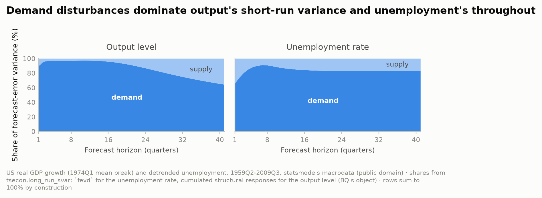
Share of the h-step forecast-error variance due to the demand
disturbance, in percent. The paper's output decomposition is for the
level, which the script computes from the cumulated structural responses
(Σ_{s≤h} C_s², normalized across disturbances); fevd from long_run_svar
gives the growth and unemployment columns directly.
| horizon (steps) | output level | output growth | unemployment |
|---|---|---|---|
| 1 | 89.5 | 89.5 | 65.4 |
| 2 | 95.5 | 87.2 | 73.9 |
| 4 | 97.1 | 87.0 | 85.3 |
| 8 | 96.8 | 83.8 | 90.6 |
| 12 | 97.1 | 84.0 | 86.3 |
| 20 | 92.1 | 83.7 | 83.2 |
| 40 | 65.3 | 83.5 | 83.0 |
Finding 5. Demand accounts for 89.5% of output's one-step variance and 92–97% from two to twenty quarters, declining to 65% at ten years as the supply disturbance's permanent effect accumulates — the shape of the paper's table (near-total demand dominance at short horizons, falling with the horizon) though it falls less far here. For unemployment the share rises from 65% at one step to 85–91% and stays there. Guard: growth share at one step > 0.5; level share > 0.8 at steps 1–12, lower at step 40 than at step 4 by at least 0.1, and above 0.4; unemployment share > 0.5 at one step and
0.7 from step 4; rows sum to one at 1e-12.
Historical decomposition
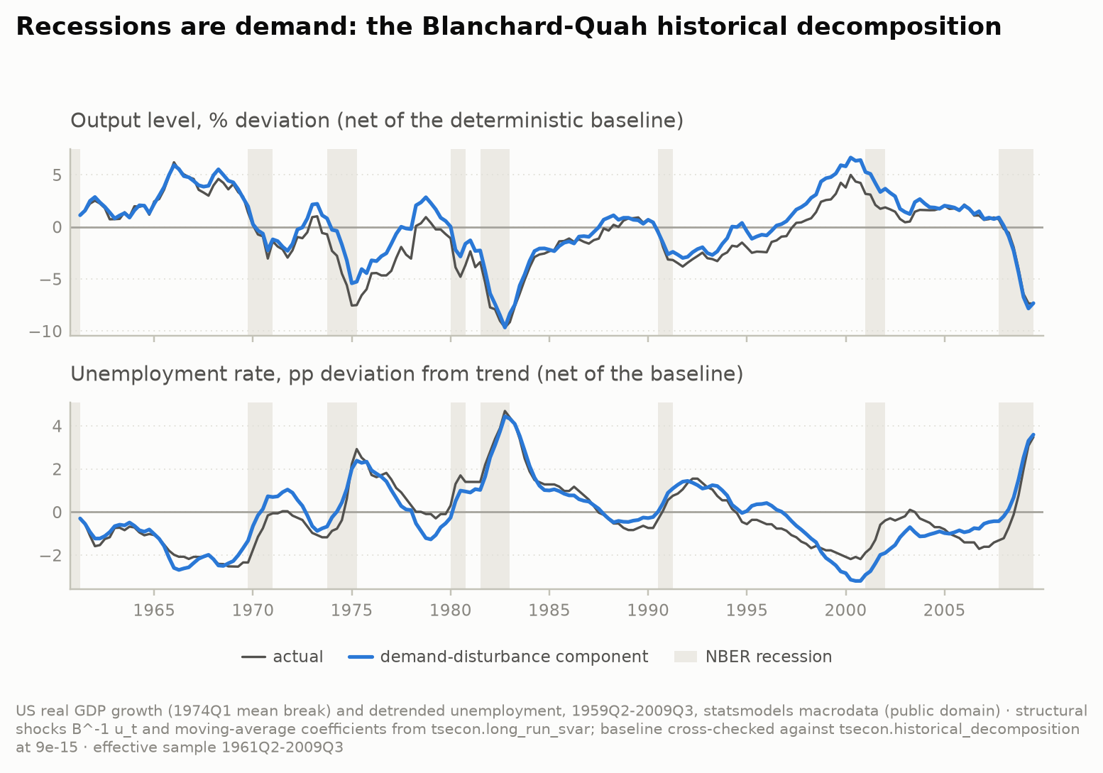
The paper's decomposition is one call, with the anchored impact matrix passed straight through (a nested list is accepted):
B = tsecon.long_run_svar(data, lags=8, impact_signs=[(0, 1)])["impact"]
hd = tsecon.historical_decomposition(data, lags=8, identification="impact", impact=B)
The reduced form is the same VAR(8) with a constant, which is the condition
for the impact matrix and the residuals to belong together. The
deterministic baseline is identification-invariant and identical to the
Cholesky decomposition's. The total shock contribution agrees to
6.2e-15, and the adding-up identity y = baseline + Σ_j hd_j holds
exactly. shock_covariance is 0.912371 times the identity, which is
\((T-m)/T\) with \(m = 17\): the df-adjusted \(\Sigma_u\) behind long_run_svar's
impact. The pre-0.11.0 construction from the structural shocks B⁻¹u_t and
the structural moving-average coefficients is kept in the script as a
cross-check (historical_decomposition_by_hand) and agrees to 3.6e-15.
The demand-disturbance component tracks detrended unemployment with a correlation of 0.926 (the supply component: 0.129), and carries the bulk of the rise in unemployment in every NBER recession inside the effective sample (1961Q2–2009Q3):
| NBER recession | rise in unemployment (pp) | demand | supply |
|---|---|---|---|
| 1969Q4–1970Q4 | +2.19 | +2.06 | +0.13 |
| 1973Q4–1975Q1 | +3.40 | +2.68 | +0.72 |
| 1980Q1–1980Q3 | +1.40 | +1.25 | +0.14 |
| 1981Q3–1982Q4 | +3.29 | +3.42 | −0.12 |
| 1990Q3–1991Q1 | +0.90 | +0.88 | +0.02 |
| 2001Q1–2001Q4 | +1.30 | +0.93 | +0.37 |
| 2007Q4–2009Q2 | +4.39 | +3.73 | +0.66 |
Recessions are demand — the reading the paper draws from its own Figures 7–8 — including the 2008–09 recession the paper could not have seen, which this identification attributes to demand at 85%. Guard: correlation > 0.8; in each of the seven recessions the demand contribution exceeds the supply contribution and more than half of the actual rise (achieved shares 0.71–1.04).
What matches the paper's procedure, and what does not
Same design. Bivariate VAR in output growth and the unemployment rate; eight lags; output growth demeaned with a break in mean at 1974Q1; unemployment linearly detrended; the long-run neutrality of demand; the objects reported — cumulated output responses, unemployment responses, variance decompositions of the output level and of unemployment, and the historical decomposition of both.
Different data. Real GDP (2005-dollar chained) over 1959Q1–2009Q3 in place of real GNP over 1948Q2–1987Q4. The estimation sample (1961Q2–2009Q3, 194 observations after eight lags) overlaps the paper's for 27 years and adds 22 more. That is why the page is graded a design replication: the shapes are the claim, not the numbers.
Different bands. The paper reports one-standard-deviation Monte Carlo
bands. This page reports long_run_svar_bands' 68%/90% residual-bootstrap
percentile bands, uncorrected for bias in the main table, with the Kilian and
delta arms beside them and their measured per-cell coverage.
Where the shapes differ. Two of the paper's finer readings are not reproduced on this vintage and are not pinned: the supply effect on output rises to its plateau non-monotonically (a dip toward zero at h = 8), and unemployment's response to a supply disturbance never turns materially negative. Demand's share of output variance at ten years (65%) is also higher than the paper's long-horizon share.
Sensitivity — what the design hinges on. Every cell below is a full
re-fit; p is the lag order (8 = the paper, 2 and 3 = BIC/HQ and AIC).
| treatment | p | y←d impact | y←d peak (h) | y←d h = 40 | y←s impact | y←s long run | u←d h = 0 | u←s h = 0 | demand share at step 4: output | unemployment |
|---|---|---|---|---|---|---|---|---|---|---|
| constant only | 2 | +0.55 | +0.97 (4) | −0.001 | +0.58 | +0.56 | −0.24 | +0.03 | 59 | 98 |
| constant only | 3 | +0.43 | +0.74 (2) | +0.008 | +0.66 | +0.59 | −0.24 | −0.02 | 37 | 86 |
| constant only | 8 | +0.43 | +0.77 (3) | −0.012 | +0.64 | +0.72 | −0.23 | −0.00 | 40 | 88 |
| mean break only | 2 | +0.75 | +1.11 (3) | −0.001 | +0.22 | +0.53 | −0.20 | +0.14 | 98 | 82 |
| mean break only | 3 | +0.73 | +1.12 (3) | +0.008 | +0.24 | +0.45 | −0.20 | +0.14 | 96 | 88 |
| mean break only | 8 | +0.71 | +1.10 (3) | −0.004 | +0.24 | +0.48 | −0.19 | +0.14 | 97 | 85 |
| detrended u only | 2 | +0.57 | +0.99 (4) | −0.001 | +0.56 | +0.56 | −0.24 | +0.03 | 62 | 99 |
| detrended u only | 3 | +0.45 | +0.77 (2) | +0.007 | +0.65 | +0.58 | −0.24 | −0.01 | 41 | 88 |
| detrended u only | 8 | +0.45 | +0.81 (3) | −0.013 | +0.63 | +0.72 | −0.23 | +0.01 | 44 | 91 |
| both (BQ) | 2 | +0.75 | +1.11 (3) | −0.001 | +0.22 | +0.53 | −0.20 | +0.14 | 98 | 83 |
| both (BQ) | 3 | +0.73 | +1.11 (3) | +0.008 | +0.25 | +0.45 | −0.20 | +0.13 | 95 | 89 |
| both (BQ) | 8 | +0.71 | +1.10 (3) | −0.004 | +0.24 | +0.48 | −0.19 | +0.14 | 97 | 85 |
The hump, its vanishing, the permanent supply effect and the negative unemployment impact survive every cell; the lag order barely matters. The break in mean growth is what the design hinges on: without it the long-run restriction reads the post-1973 slowdown as one enormous supply disturbance, the supply impact on output doubles, the positive supply-on-unemployment impact disappears, and demand's share of output variance a year out collapses from 97% to about 40%. That is the Faust-Leeper point made concrete — a long-run restriction inherits every low-frequency feature of the data you did not model — and it is why the paper spends a section on this choice. Detrending unemployment, by contrast, changes nothing of substance.
Library gaps this page used to work around, now closed (0.11.0). Before
0.11.0, long_run_svar had no native confidence bands and
historical_decomposition had no arbitrary-impact-matrix entry point. Both
objects were built in the script from shipped primitives (var_fit,
bootstrap_indices, long_run_svar). They are now long_run_svar_bands and
historical_decomposition(identification="impact"), and the old
constructions remain only as cross-checks, at the agreement quoted above.
Cross-check: the closed form, independently
The identification itself is dual-checked on this data: an independent NumPy
transcription of the Blanchard-Quah closed form on a statsmodels
VAR(data).fit(8) — C(1) = (I − ΣAᵢ)⁻¹, LR = chol(C(1) Σ C(1)ᵀ),
B = C(1)⁻¹ LR, with the df-adjusted sigma_u and the same demand-column
sign — agrees with long_run_svar to 2.0e-13 on B, 2.5e-12 on the
long-run matrix and 6.4e-12 on C(1) (guard: 1e-9). The same transcription underlies the crate's golden
fixture (long_run_svar.json); here it
is run on real data rather than a synthetic system.
What is being claimed. This reproduces Blanchard-Quah's economics on a later vintage of the same two US series — two disturbances with the published dynamic signatures, the published ordering of variance shares, and recessions that are demand — with every shape pinned to a stated band, and the identification step verified against an independent implementation to machine precision. It does not claim that any number matches a 1989 table, and it says where the shapes differ.
Citation. Blanchard, O. J. and D. Quah (1989), "The Dynamic Effects of
Aggregate Demand and Supply Disturbances," American Economic Review
79(4):655–673. Read alongside Faust, J. and E. M. Leeper (1997), "When Do
Long-Run Identifying Restrictions Give Reliable Results?", Journal of
Business & Economic Statistics 15(3):345–353. Data: US-government statistics
(public domain), from statsmodels' bundled macrodata.
See also. long_run_svar model card ·
identification guide ·
Uhlig replication ·
Gertler-Karadi replication.