Chapter 2 — Exploring and Diagnosing a Series
Part of The tsecon Guide to Time Series Econometrics. Chapters mirror the library's modules; code runs against the current Python API unless marked otherwise.
Prerequisites: Chapter 1's vocabulary — stationarity, autocovariance, white noise — plus basic OLS regression.
You will learn:
- How to read ACF and PACF plots the way a practitioner does, including the signature table that maps patterns to model families
- How to test whether residuals are white noise (Ljung-Box), normal (Jarque-Bera), and free of volatility clustering (Engle's ARCH-LM)
- How unit-root testing actually works — ADF mechanics, why lag and deterministic choices decide the outcome, and why KPSS must run alongside it
- The confirmatory quadrant workflow, and how
check_stationaritycodifies it - How to hunt structural breaks up the full ladder — a known date (Chow), monitoring (CUSUM), an unknown date (sup-F), and multiple breaks with confidence intervals (Bai-Perron)
- Where seasonality detection and spectral analysis fit in — and what is still on the roadmap
The idea
You have just loaded a series — say, a century of annual river flows, or forty years of quarterly GDP. The worst thing you can do next is fit a model. The best thing you can do is interrogate the data, the way a doctor runs tests before writing a prescription.
Every question in this chapter is a version of one master question: what structure does this series carry, and is that structure stable enough to model? Concretely:
- Does the past predict the future? If this quarter's GDP growth is high, is next quarter's likely to be high too? The autocorrelation function answers this lag by lag, and the pattern of its answer tells you what family of model to reach for.
- Is the level of the series anchored? Unemployment wanders but keeps returning to a band; the price level never returns anywhere — it drifts forever. These two kinds of series need fundamentally different treatment, and confusing them is the most expensive mistake in applied time series work. The unit-root tests in this chapter exist to tell them apart.
- Does the series breathe with the calendar? Retail sales spike every December. A model that ignores this will be wrong twelve times a year, on schedule.
- Did the world change partway through? A policy regime shift or a war can snap the parameters of the data-generating process. A single model fit across the break averages two different worlds and describes neither.
Picture the two plots you will make first. For a mean-reverting series, the autocorrelation plot looks like a staircase descending quickly to zero: the past matters, but its grip fades. For a drifting series like the price level, the staircase barely descends at all — the bars start near one and melt down almost linearly, a visual confession that shocks never die out. Learning to see that difference at a glance, and then to confirm it with formal tests rather than trusting your eyes, is what this chapter teaches.
Everything downstream — ARIMA in the univariate chapters, VARs in the multivariate ones, GARCH in the volatility chapter — consumes the verdicts made here. This is the base layer of the library and of your workflow.
Reading the ACF and PACF
Why you care. The autocorrelation function (ACF) and partial autocorrelation function (PACF) are the fingerprint of a series. In the Box-Jenkins tradition (Box and Jenkins, 1970) they are the model-identification step: their joint pattern tells you whether the series behaves like an autoregression, a moving average, a mix, a seasonal process — or something you must transform before modeling at all.
The formalism. For a covariance-stationary series \(y_t\) with mean \(\mu\), the autocovariance at lag \(k\) and the autocorrelation are
so \(\rho_k\) is the correlation between the series and itself \(k\) periods ago; \(\rho_0 = 1\) always. The sample version replaces moments with averages:
Note the divisor \(T\), not \(T-k\): this "biased" estimator guarantees the autocovariance sequence is positive semidefinite (a valid covariance structure), and it is what R and statsmodels use. tsecon follows the same convention.
Two kinds of confidence band exist, and they answer different questions:
- White-noise band \(\pm 1.96/\sqrt{T}\): under the null that the series is white noise (no autocorrelation at any lag), each \(\hat\rho_k\) is approximately \(N(0, 1/T)\). Use this band on residuals, where white noise is the hypothesis you care about.
- Bartlett band (Bartlett, 1946): under the null that the series is MA(\(k-1\)) — correlated up to lag \(k-1\), zero beyond — the variance of \(\hat\rho_k\) is approximately \(\bigl(1 + 2\sum_{j=1}^{k-1}\hat\rho_j^2\bigr)/T\), which is wider than the white-noise band. Use this when asking "does correlation extend past lag \(q\)?" — the MA order-selection question.
The PACF at lag \(k\), written \(\phi_{kk}\), is the correlation between \(y_t\) and \(y_{t-k}\) after removing the influence of the intervening observations \(y_{t-1}, \dots, y_{t-k+1}\). Equivalently, it is the coefficient on \(y_{t-k}\) in a regression of \(y_t\) on its first \(k\) lags. For an AR(\(p\)) process the PACF is exactly zero beyond lag \(p\) — that is the whole trick.
import numpy as np
import tsecon

# An AR(2): y_t = 1.3 y_{t-1} - 0.4 y_{t-2} + eps_t
rng = np.random.default_rng(42)
n = 400
y, eps = np.zeros(n), rng.normal(size=n)
for t in range(2, n):
    y[t] = 1.3 * y[t - 1] - 0.4 * y[t - 2] + eps[t]

r = tsecon.acf(y, nlags=24)        # dict: acf, bartlett_se
p = tsecon.pacf(y, nlags=24)       # Yule-Walker ("yw") or "ols"

r["acf"][1:4]                      # [0.912, 0.751, 0.585] — smooth decay
p[1:4]                             # [0.912, -0.476, 0.062] — two spikes, then dead
band = 1.96 / np.sqrt(len(y))      # 0.098 — the white-noise band
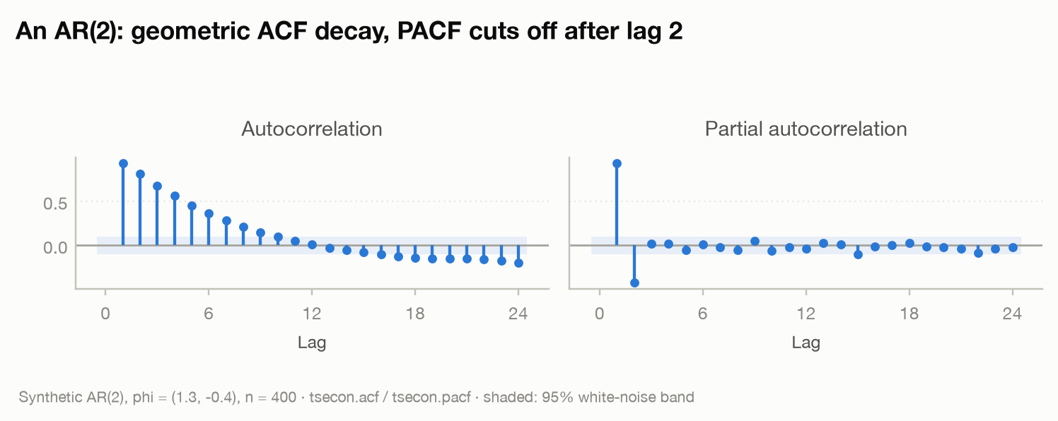
The figure shows the pattern you should learn to recognize on sight: the ACF decays geometrically (with a hint of oscillation from the second-order dynamics), while the PACF shows exactly two significant spikes and then dies. Read "fit an AR(2)" straight off the plot.
The signature table. Memorize this — it is the practitioner's decoder ring:
| Series type | ACF pattern | PACF pattern |
|---|---|---|
| AR(\(p\)) | Geometric decay (possibly oscillating) | Cuts off sharply after lag \(p\) |
| MA(\(q\)) | Cuts off sharply after lag \(q\) | Geometric decay |
| ARMA(\(p,q\)) | Decay beginning after lag \(q\) | Decay beginning after lag \(p\) |
| Seasonal (period \(s\)) | Spikes at lags \(s, 2s, 3s, \dots\) | Spike(s) at seasonal lags |
| Nonstationary (unit root) | Starts near 1, decays almost linearly, stays high for dozens of lags | Single enormous spike at lag 1, near 1 |
| White noise | Nothing outside the band at any lag | Nothing outside the band |
The last two rows are the guardrails. A near-linear, slow-melting ACF is not an invitation to fit a very long AR — it is a symptom that the series has no fixed mean to revert to, and you should go straight to the unit-root tests below. And a clean white-noise fingerprint on your residuals is the certificate every fitted model must earn.
⚠ Common mistake. Using the wrong band. The \(\pm 1.96/\sqrt{T}\) band tests "white noise at every lag"; the Bartlett band tests "no correlation beyond lag \(k\)." They can disagree, and plotting one while reasoning about the other inverts conclusions — a lag can sit outside the white-noise band yet inside the Bartlett band. tsecon returns
bartlett_seexplicitly so you always know which one you are drawing.
Portmanteau tests: is anything left?
Why you care. Eyeballing twenty ACF bars invites cherry-picking: with twenty bars and a 95% band, one bar sticks out by chance alone. A portmanteau ("suitcase") test packs the first \(h\) autocorrelations into a single statistic with a single p-value. Its main job in practice is residual checking: after fitting a model, the residuals should be white noise — serially uncorrelated, with constant mean and variance — meaning the model has absorbed all the linear predictability. Correlated residuals mean predictability left on the table and standard errors you cannot trust.
The formalism. The Box-Pierce statistic (Box and Pierce, 1970) and its small-sample refinement, the Ljung-Box statistic (Ljung and Box, 1978), are
Under the null of white noise, both are asymptotically \(\chi^2_h\). The Ljung-Box weights upweight higher lags to correct the finite-sample downward bias of \(\hat\rho_k\); it is the default everywhere, including here.
e = rng.normal(size=300)           # white noise: the test should pass
lb = tsecon.ljung_box(e, nlags=12) # dict: lags, lb_stat, lb_pvalue, bp_stat, bp_pvalue
lb["lb_pvalue"][-1]                # 0.80 — no evidence against whiteness

lb_ar = tsecon.ljung_box(y, nlags=12)   # the AR(2) from above
lb_ar["lb_pvalue"][0]              # ~1e-75 — emphatically not white noise
The function returns the cumulative statistic and p-value at every lag from 1 to nlags, so you can see where the correlation lives, not just that it exists.
⚠ Common mistake. Degrees of freedom on residuals. When \(Q_{LB}(h)\) is computed on the residuals of a fitted ARMA(\(p,q\)) model, the correct reference distribution is \(\chi^2_{h-p-q}\), not \(\chi^2_h\) — estimating the model soaks up \(p+q\) degrees of freedom. tsecon's
ljung_boxis a raw-series test (df \(= h\)); on ARMA residuals, comparelb_stat[h-1]to a \(\chi^2_{h-p-q}\) critical value yourself. (A fitted-model-aware residual battery is on the Module 01 roadmap.) A second trap: the test is invalid on GARCH-standardized residuals — the estimation effect changes the null distribution, and the Li-Mak test is the correct tool there.
Model-adequacy checks: normality and ARCH effects
Why you care. White-noise residuals are necessary but not sufficient. Two further checks matter before you trust a model's intervals and density forecasts. First, normality: prediction intervals and likelihood-based inference typically assume Gaussian errors. Second — and specific to economics and finance — ARCH effects: the tendency of volatility to cluster, with calm months following calm months and turbulent months following turbulent ones. Stock returns are the canonical case: their levels are nearly uncorrelated, but their squares are strongly autocorrelated. A series can pass Ljung-Box on levels and be wildly non-white in its variance. The converse trap matters too: Ljung-Box's null is iid noise, so volatility clustering alone can make it reject on returns that are in fact uncorrelated. When the real question is whether a price is a random walk — whether its increments are serially uncorrelated at all — variance_ratio(log_price) asks it directly, with a statistic that stays valid under ARCH (see the variance-ratio model card).
Jarque-Bera (Jarque and Bera, 1980) tests normality through the third and fourth moments. With sample skewness \(S\) and kurtosis \(K\) (Gaussian values 0 and 3),
Fat tails (\(K > 3\)) or asymmetry (\(S \neq 0\)) inflate the statistic.
Engle's ARCH-LM test (Engle, 1982) regresses squared residuals on their own lags:
and under the null of no ARCH (all \(\alpha_i = 0\)), the Lagrange-multiplier statistic \(T \cdot R^2\) from this auxiliary regression is \(\chi^2_q\). Rejection is the gateway diagnostic to the GARCH chapter: it says the variance itself is forecastable.
jb = tsecon.jarque_bera(e)
jb["p_value"], jb["skewness"], jb["kurtosis"]   # 0.95, -0.01, 2.91 — Gaussian looks fine

# Simulate an ARCH(1): calm and turbulent spells cluster
a, sig2, z = np.zeros(500), np.ones(500), rng.normal(size=500)
for t in range(1, 500):
    sig2[t] = 0.2 + 0.7 * a[t - 1] ** 2
    a[t] = np.sqrt(sig2[t]) * z[t]

tsecon.arch_lm(a, nlags=4)["p_value"]   # ~0.0000 — strong ARCH, go fit a GARCH
tsecon.arch_lm(e, nlags=4)["p_value"]   # 0.66   — iid noise, nothing there
⚠ Common mistake. Overreacting — or underreacting — to a normality rejection. Non-normal errors do not invalidate your coefficient estimates (OLS and quasi-maximum-likelihood point estimates remain consistent); they invalidate Gaussian prediction intervals and density forecasts. Conversely, in samples of a few thousand, JB rejects for economically trivial departures. Also note JB's asymptotic \(\chi^2_2\) approximation is famously poor in small samples — the roadmap adds simulated small-sample p-values. And as with Ljung-Box: ARCH-LM applied to standardized residuals of an already-fitted GARCH model is invalid; that is Li-Mak territory.
Unit roots done right: the ADF test
Why you care. Regress one drifting series on another, unrelated drifting series, and OLS will report a large \(t\)-statistic and a high \(R^2\) most of the time — the spurious regression problem (Granger and Newbold, 1974; formalized by Phillips, 1986). The culprit is the unit root: a series whose shocks accumulate forever instead of decaying, like a random walk \(y_t = y_{t-1} + \varepsilon_t\). Such a series is called integrated of order one, I(1); differencing it once yields a stationary, I(0), series. Before any regression or ARMA fit, you must know which side of that line your series is on — and eyeballing cannot settle it, because a stationary series with a root of 0.97 and a true random walk look nearly identical over typical macro samples.
The formalism. The Dickey-Fuller idea (Dickey and Fuller, 1979) is to regress the change in the series on its own lagged level. The augmented version (ADF) adds lagged differences to soak up short-run serial correlation:
The null hypothesis is \(\gamma = 0\): the level has no pull on the change, so shocks never revert — a unit root. The alternative is \(\gamma < 0\): the series is pulled back toward its mean (or trend), i.e., stationary. Three ingredients decide whether the test works:
- The lags \(\sum \delta_i \Delta y_{t-i}\). Without them, serial correlation in \(\varepsilon_t\) wrecks the test's size. With too many, power evaporates. tsecon selects \(p\) automatically by AIC (default), BIC, or the sequential \(t\)-significance rule, or you can fix it.
- The deterministics \(\alpha\) and \(\beta t\). Choose the specification that describes the series under the alternative you care about:
"c"(constant) when a stationary series would fluctuate around a nonzero level;"ct"(constant + trend) when the plausible alternative is stationary fluctuation around a deterministic trend line — GDP being the classic case;"n"(neither) almost never. This choice changes the critical values and the power, in both directions — see the trap below. - The p-values. Under the null, the \(t\)-statistic on \(\hat\gamma\) does not follow a \(t\) distribution — it follows the nonstandard Dickey-Fuller distribution, shifted left, with critical values near \(-2.9\) (constant case) rather than \(-1.96\). tsecon computes p-values from the MacKinnon response surfaces (MacKinnon, 1996, 2010) — regression-smoothed simulations that adjust for your exact sample size — never from the coarse original tables.
rw = np.cumsum(rng.normal(size=300))          # a pure random walk

res = tsecon.adf(rw, regression="c")           # constant; lags by AIC (default)
res["statistic"], res["p_value"]               # -2.08, 0.25 — cannot reject the unit root
res["used_lag"], res["nobs"]                   # 0 lags chosen, 299 usable obs
res["crit"]["5%"]                              # -2.87 — the MacKinnon critical value

tsecon.adf(rw, regression="ct", autolag="bic") # trend case, BIC lag selection
tsecon.adf(rw, regression="c", autolag=None, maxlag=4)  # fixed 4 lags

tsecon.adf(y, regression="c")["p_value"]       # ~1e-9 — the AR(2) is confidently stationary
Note what a failure to reject means: not "this series has a unit root," but "we could not tell it apart from one." Unit-root tests have notoriously low power against nearby alternatives — a fact the confirmatory workflow below is designed to confront.
⚠ Common mistake. Treating the deterministic specification as a nuisance detail. It is the whole game. Include a trend the data do not need and you throw away power: on the level-drifting series in the worked example below,
regression="c"gives \(p = 0.06\) while an unnecessaryregression="ct"gives \(p = 0.62\) — same data, opposite verdicts. Omit a trend the data do have and the test cannot reject a unit root against the trend-stationary truth no matter how much data you collect. Plot the series, decide what the stationary alternative would look like, and match the specification to it. And never look up a plain \(t\) table: \(-2.5\) is "significant" in a \(t\) world and nothing at all in the Dickey-Fuller world.
The Phillips-Perron alternative: correct for serial correlation without lags
ADF soaks up serial correlation by adding lagged differences — and you must choose how many. Phillips and Perron (1988) take the other route: run the plain Dickey-Fuller level regression with no augmentation, then correct the statistic itself for serial correlation using a kernel (Bartlett) estimate of the residual's long-run variance — the same HAC machinery behind Newey-West standard errors and the KPSS denominator below. The null (a unit root), the nonstandard Dickey-Fuller distribution, and the MacKinnon p-values are all identical to ADF; only the nuisance-correction differs. phillips_perron ships it, matching arch.unitroot.PhillipsPerron to machine precision:
rng_pp = np.random.default_rng(0)
walk = np.cumsum(rng_pp.standard_normal(300))     # a random walk (unit root)
noise = rng_pp.standard_normal(300)               # i.i.d. (stationary)

pp = tsecon.phillips_perron(walk, regression="c")            # test_type="tau" (Z-tau) is the default
pp_noise = tsecon.phillips_perron(noise)
print("PP(walk)  Z-tau:", round(pp["stat"], 4), " p:", round(pp["pvalue"], 4),
      " bandwidth:", pp["lags"])
print("PP(noise) Z-tau:", round(pp_noise["stat"], 4), " p:", round(pp_noise["pvalue"], 4))
The random walk cannot reject the unit root; the i.i.d. series rejects overwhelmingly. Use PP as a robustness cross-check on ADF — agreement is reassuring — but it inherits ADF's low power near the boundary and its size distortion under a large negative MA root, so it does not replace the confirmatory ADF+KPSS quadrant below. The same semiparametric correction, applied to the residual of a cointegrating regression, gives phillips_ouliaris — the single-equation cointegration test (null: no cointegration); see the model card.
KPSS and the confirmatory quadrant
Why you care. ADF puts the unit root under the null, so it is conservative toward finding unit roots: with low power, "cannot reject" is weak evidence. The KPSS test (Kwiatkowski, Phillips, Schmidt and Shin, 1992) flips the burden of proof: its null is stationarity, its alternative a unit root. Running both gives you two independent angles on the same question, and only their agreement deserves your confidence. This confirmatory logic is standard advice in every textbook and implemented almost nowhere — tsecon ships it as check_stationarity.
The formalism. KPSS decomposes the series as \(y_t = \xi t + r_t + \varepsilon_t\), where \(r_t = r_{t-1} + u_t\) is a random-walk component with variance \(\sigma^2_u\). The null \(H_0: \sigma^2_u = 0\) says the walk is frozen — the series is stationary around a level (regression="c") or a trend (regression="ct"). The statistic accumulates the partial sums of the demeaned (or detrended) residuals \(\hat e_t\):
where \(\hat\lambda^2\) is the long-run variance of \(\hat e_t\) — a HAC estimate (the same machinery behind Newey-West standard errors; see tsecon.long_run_variance) whose bandwidth choice materially moves the statistic. tsecon defaults to the Hobijn-Franses-Ooms automatic bandwidth and reports the lags used, because a KPSS result quoted without its bandwidth is not reproducible.
k = tsecon.kpss(rw, regression="c")     # the random walk from above
k["statistic"], k["p_value"], k["lags"] # 0.77, 0.01, 10 — rejects stationarity
tsecon.kpss(y, regression="c")["p_value"]   # 0.10 — the AR(2) passes
tsecon.kpss(y, regression="ct", nlags="legacy")  # trend null, legacy bandwidth
KPSS p-values come from a sparse published table covering only \([0.01, 0.10]\); tsecon interpolates within it and clamps at the edges, statsmodels-style — so p_value == 0.01 means "at most 0.01."
The quadrant. Two tests, two possible verdicts each, four cells:
| KPSS does not reject (looks stationary) | KPSS rejects (not stationary) | |
|---|---|---|
| ADF rejects (no unit root) | Stationary — both agree: proceed in levels | Conflict — trend, structural breaks, or long memory; not a clean I(0)/I(1) case |
| ADF does not reject (unit root plausible) | Inconclusive — both nulls survive: low power, likely too little data | UnitRoot — both agree: difference once and re-test |
check_stationarity runs both tests and hands you the cell, a recommendation, and a plain-language interpretation:
rep = tsecon.check_stationarity(rw)     # optional: alpha=0.10
rep["quadrant"]          # "UnitRoot"
rep["recommendation"]    # "Difference"
rep["interpretation"]    # a paragraph explaining the evidence
rep["adf_p_value"], rep["kpss_p_value"]
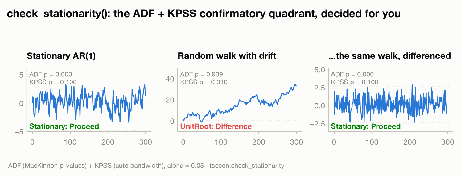
The figure walks the full loop: a stationary AR(1) (both tests agree — proceed), a random walk with drift (both agree — difference), and the differenced walk (proceed) — the workflow closes.
⚠ Common mistake. Running ADF alone and stopping. "ADF failed to reject, so I differenced" is the single most common stationarity error: with \(T = 100\) and a root of 0.95, ADF fails to reject most of the time even though the series is stationary — and differencing a stationary series (overdifferencing) injects an artificial MA unit root that degrades every model fit afterward. The quadrant exists precisely to catch this: that case lands in Inconclusive, not UnitRoot, telling you the honest answer is "the data cannot settle it," not "difference."
A full diagnostic pass: a Nile-like series
Time to run the whole battery on one series and read the results together. The synthetic series below mimics the famous Nile riverflow data (annual flows, 1871–1970, the canonical example in the state-space literature): an unobserved level that wanders slowly — a random walk with small innovations — buried in large measurement noise. The variances are set to the maximum-likelihood values estimated on the real Nile.
import numpy as np
import tsecon

rng = np.random.default_rng(7)
T = 100
mu = 919.0 + np.cumsum(rng.normal(0.0, 38.0, T))   # slowly wandering true level
nile = mu + rng.normal(0.0, 123.0, T)              # observed flow: level + noise

# --- Step 1: is it stationary? ---
rep = tsecon.check_stationarity(nile)
rep["quadrant"], rep["recommendation"]   # ("UnitRoot", "Difference")
rep["adf_p_value"], rep["kpss_p_value"]  # (0.062, 0.01) — both point the same way

# --- Step 2: difference, and re-run the loop ---
d = np.diff(nile)
tsecon.check_stationarity(d)["quadrant"]   # "Stationary" — proceed

# --- Step 3: what dependence is left in the differences? ---
r = tsecon.acf(d, nlags=10)
r["acf"][1:4]                    # [-0.54, 0.03, 0.03] — one spike, then nothing
tsecon.pacf(d, nlags=10)[1:5]    # [-0.54, -0.37, -0.24, -0.11] — geometric decay
lb = tsecon.ljung_box(d, nlags=10)
lb["lb_pvalue"][-1]              # 5e-6 — stationary, but NOT white noise

# --- Step 4: adequacy checks on the differences ---
tsecon.jarque_bera(d)["p_value"]              # 0.89 — no evidence against normality
tsecon.arch_lm(d - d.mean(), nlags=4)["p_value"]  # 0.10 — no clear ARCH
Now read the evidence like a practitioner:
- Levels: ADF cannot reject a unit root (\(p = 0.062\)) and KPSS rejects stationarity (\(p \le 0.01\)). Both tests point the same way — the UnitRoot cell. Difference once.
- Differences: the quadrant says Stationary, but Ljung-Box emphatically rejects whiteness (\(p \approx 10^{-5}\)). Stationary is not the same as unpredictable — there is structure left to model.
- What structure? The ACF of the differences cuts off sharply after one large negative spike (\(\hat\rho_1 = -0.54\)) while the PACF decays geometrically. Read that off the signature table: MA(1). So the original series behaves like an ARIMA(0,1,1) — which is exactly the reduced form of the local-level model that generated it (and which Chapter 1's
local_level_smoothcan filter directly). The diagnostics have reverse-engineered the data-generating process. - Adequacy: normal errors, no ARCH. Gaussian prediction intervals will be honest, and there is no volatility clustering to chase.
This is the base-layer workflow in miniature: quadrant → transform → fingerprint → adequacy, every arrow driven by a test rather than a hunch.
⚠ Common mistake. Misreading the big negative spike. A lag-1 autocorrelation near \(-0.5\) in a differenced series has two readings: a genuine MA(1) after correct differencing (as here — noise-dominated level series imply \(\hat\rho_1\) between \(-0.5\) and \(0\)), or the scar of overdifferencing a series that was already stationary (\(\hat\rho_1 \to -0.5\) exactly, an MA root of one). The closer the spike sits to \(-0.5\), the more seriously you should revisit step 1 — which is why the quadrant, not the ACF, makes the differencing call.
Detecting seasonality
Why you care. Monthly and quarterly economic series — retail sales, employment, industrial production — carry calendar rhythms that dwarf the fluctuations you actually want to study. Detecting seasonality is cheap; ignoring it poisons every downstream diagnostic (a seasonal pattern looks like strong autocorrelation to Ljung-Box and can distort unit-root tests).
The first-line detector is the ACF itself: seasonality shows up as spikes at the seasonal lags \(s, 2s, 3s, \dots\) — 12 and 24 for monthly data, 4 and 8 for quarterly:
# A monthly series with an annual cycle
pattern = np.array([5, 3, 1, -2, -4, -6, -5, -3, 0, 2, 4, 6], dtype=float)
ts = np.tile(pattern, 10) + rng.normal(0, 1.0, 120)

sa = tsecon.acf(ts, nlags=25)
sa["acf"][12], sa["acf"][24]     # 0.84, 0.76 — unmistakable annual spikes
Detection is only step one; the harder question is what kind of seasonality you found, because the remedy differs:
- Deterministic seasonality — the same fixed pattern every year — is handled with seasonal dummy variables or harmonic regressors, leaving the series otherwise intact.
- Stochastic seasonality — a seasonal pattern that itself drifts over time (a seasonal unit root) — requires seasonal differencing (\(y_t - y_{t-s}\)).
Distinguishing them is the job of the HEGY test (Hylleberg, Engle, Granger and Yoo, 1990), which tests for unit roots at the zero frequency and at each seasonal frequency separately, and of the Canova-Hansen test (Canova and Hansen, 1995), which — KPSS-style — takes stable seasonality as its null. Both are on the Module 01 roadmap, alongside the QS test (the X-13 residual-seasonality workhorse) and the Friedman and Kruskal-Wallis rank tests; none of the four has a credible Python implementation today, and HEGY in particular is a headline gap the library aims to fill.
What does ship is the decision rule practitioners actually reach for. tsecon.stl (and tsecon.mstl for multiple periods) decomposes the series; tsecon.seasonal_strength reads the Wang-Smith-Hyndman strength off that decomposition; and tsecon.nsdiffs turns the strength into a verdict — the forecast::nsdiffs(test="seas") rule, differencing at the seasonal lag while the strength stays at or above 0.64:
ns = tsecon.nsdiffs(ts, period=12)
ns["d"], ns["stop"]                      # 1 'WeakSeasonality' — one seasonal difference, then done
ns["steps"][0]["seasonal_strength"]      # 0.96 — the strength that triggered it
tsecon.seasonal_strength(ts, period=12)["seasonal_strength"]   # 0.96, the same number standalone
That is a strength threshold, not a hypothesis test — it answers "is the seasonality strong enough that differencing helps?", not "is there a seasonal unit root?" The second question is what HEGY and Canova-Hansen are for, and it is the one still open.
⚠ Common mistake. Seasonally differencing on sight. Applying \(y_t - y_{t-s}\) to a series whose seasonality is deterministic overdifferences it at every seasonal frequency — the seasonal analogue of the trap in the previous section. The choice between dummies and seasonal differences is a testing question (HEGY/Canova-Hansen), not a reflex.
Structural breaks: when the parameters move
Why you care. Every test so far assumes one data-generating process throughout the sample. But economies get reorganized: the 1973 oil shock, the Volcker disinflation, the euro, COVID. If the mean, trend, or dynamics shifted partway through your sample, a single-model fit describes neither regime — and, more insidiously, a stationary series with a broken mean is nearly observationally equivalent to a unit-root series. Perron (1989) showed that standard ADF tests, applied to series that are stationary around a broken trend, fail to reject a unit root almost always. A chunk of the "unit roots in macro" literature is arguably about unmodeled breaks.
The conceptual toolkit, in ascending order of ambition:
- Chow test (Chow, 1960): you know the candidate break date; fit the model on each side and F-test whether the coefficients differ.
- CUSUM (Brown, Durbin and Evans, 1975): you suspect instability but have no date; monitor the cumulative sum of recursive residuals and flag when it drifts outside probabilistic boundaries. A drifting CUSUM path is the classic picture of a model quietly going stale.
- Quandt-Andrews sup-Wald (Andrews, 1993): compute the Chow statistic at every plausible date and take the maximum. Because you searched, the maximum's distribution is nonstandard — critical values come from Hansen's (1997) approximations.
- Bai-Perron (Bai and Perron, 1998, 2003): the full solution — estimate the number and locations of multiple breaks by dynamic programming over all partitions, with confidence intervals for each break date. Long the headline gap in every Python stack; tsecon ships it.
The entire ladder is callable today — Chow and CUSUM alongside the rest of the specification-test battery (see the specification-tests model card), sup-F and Bai-Perron in the break suite proper (see the structural-breaks model card). Walk it end to end on a series built to have two mean breaks:
rng = np.random.default_rng(42)
T = 300
mu = np.where(np.arange(T) < 100, 0.0, np.where(np.arange(T) < 200, 2.0, 0.5))
y_brk = mu + rng.normal(0.0, 1.0, T)   # white noise around a mean that jumps twice
X = np.ones((T, 1))                    # mean-shift model: every coefficient switches

# The Perron trap, live: this stationary series FAILS the unit-root screen.
rep = tsecon.check_stationarity(y_brk)
rep["quadrant"]                        # "UnitRoot" — wrong, and confidently so
rep["adf_p_value"], rep["kpss_p_value"]  # (0.057, 0.021) — both point the same (wrong) way
The quadrant workflow from earlier in this chapter — run in good faith — recommends differencing a series that is white noise around a broken mean. That is Perron's warning made concrete, and it is why the break ladder belongs in the diagnostic pass, not in an appendix.
Rung 1 — you know the date. If history hands you the candidate break (a policy change, a war), chow_test is sharp:
Rung 2 — you merely suspect instability. CUSUM monitors the recursive residuals with no date in hand:
cs = tsecon.cusum_test(y_brk, X)
((cs["path"] > cs["bound_upper"]) | (cs["path"] < cs["bound_lower"])).any()   # True — drifted out
Rung 3 — one unknown date, with honest inference. sup_f_test computes the Chow F at every admissible date (15% trimming by default) and takes the supremum, with Hansen's (1997) response-surface p-value that correctly prices the search:
sf = tsecon.sup_f_test(y_brk, X, trim=0.15)
sf["stat"], sf["p_value"]   # (83.7, 3.9e-18) — decisive instability
sf["break_date"]            # 99 — the argmax of the F path: the first break, found blind
The function also returns the full f_path over the trimmed dates, which is worth plotting: a sharp single peak reads very differently from a broad plateau (one clean break versus smeared drift). Here the path towers at observation 99 — the true first break — then falls to nothing near observation 180 and rises to a second local peak (F \(\approx 13\), itself above the critical value) near observation 201. A sup-F test can only report one date; a two-humped F path is its way of telling you it was asked the wrong question, and the next rung exists for exactly that.
Rung 4 — how many breaks, where, and how sure? bai_perron solves the multi-break problem by dynamic programming over all admissible partitions (validated in the test suite against brute-force enumeration), picks the number of breaks by sequential sup-F tests at the published Bai-Perron 5% critical values, and attaches Bai (1997) confidence intervals to each estimated date:
bp = tsecon.bai_perron(y_brk, X, max_breaks=5, trim=0.15)
bp["n_breaks"]                                   # 2
bp["break_dates"]                                # [99, 201] — truth: 99 and 199
list(zip(bp["ci_lower_95"], bp["ci_upper_95"]))  # [(95, 103), (196, 206)] — both cover
[round(p[0], 2) for p in bp["params"]]           # [-0.05, 1.98, 0.42] — truth: 0.0, 2.0, 0.5
np.round(bp["sup_f_seq"][:3], 1)                 # [83.7, 121.5, 4.5]
bp["sup_f_crit"][:3]                             # [8.58, 10.13, 11.14]
Read the selection logic off the last two lines: supF(1|0) \(= 83.7 > 8.58\), so at least one break; supF(2|1) \(= 121.5 > 10.13\), so a second; supF(3|2) \(= 4.5 < 11.14\), stop. Two breaks, dated within two observations of the truth, with 95% intervals that cover — and the three regime means recovered to within sampling noise. The ssr_path (global minimum SSR for each break count) and break_dates_by_m (the optimal partition for every candidate \(m\)) come back too, so you can see the diminishing returns the sequential test formalized.
One honesty note before you cite the intervals in a paper: the confidence intervals are the Bai (1997) homogeneous case — regressors and errors assumed to have the same distribution across regimes. The heterogeneity-robust variant (regime-specific moment matrices) is not shipped; if the regimes plausibly differ in variance, read the intervals as approximate. The structural-breaks model card states the full contract, including the trim-implied minimum regime length (\(h = 45\) here — a trim of 0.15 means no regime shorter than 15% of the sample can be found, which is a modeling choice, not a numerical detail).
Back to the trap: the unit-root test that knows about breaks. The whole reason this ladder sits inside a diagnostics chapter is that check_stationarity misread y_brk as I(1). zivot_andrews is the direct repair — it searches the break date inside the unit-root regression, so the alternative it tests against is "stationary around one broken deterministic component" rather than "stationary around a constant":
za = tsecon.zivot_andrews(y_brk)          # regression="c": an intercept shift
za["stat"], za["pvalue"]                  # (-6.299, 0.0005) — the unit root is rejected
za["crit"]["1%"]                          # -5.276: past the 1% value, not a marginal call
za["break_index"]                         # 99 — the first break, found by the test itself
Same series, same data, opposite verdict: the plain quadrant said UnitRoot, and a test allowed one break says stationary with \(p = 0.0005\). Two caveats keep this honest. zivot_andrews admits exactly one break, and this series has two — it finds the first and absorbs the second into the residual, which is why the ladder above (and bai_perron in particular) is still the tool for counting them. And its p-values interpolate a simulated table, so read at most two decimals into them.
⚠ Common mistake. Concluding "unit root" from ADF without ever asking about breaks. The two-break example above did exactly that on purpose:
check_stationarityreturned UnitRoot on a series that is white noise around a broken mean, and onlybai_perrontold the truth. The Conflict cell of the quadrant (ADF rejects, KPSS rejects) is often the same signature — and so is a stubborn non-rejection on a series with an obvious level shift. Whenever the quadrant surprises you, runsup_f_testbefore you difference — or run the unit-root test that already knows about breaks:tsecon.zivot_andrewsputs one endogenous break inside the null-hypothesis machinery, so a stationary series around a broken mean is no longer forced to read as I(1). Break-robust unit-root tests exist because the plain ADF verdict is unreliable in the presence of breaks; the two-break Lee-Strazicich (2003) extension is still a roadmap item.
The spectrum: variance, frequency by frequency
Why you care. Everything above works in the time domain — correlations across lags. The frequency domain asks a complementary question: of the series' total variance, how much comes from slow cycles and how much from fast wiggles? For business-cycle economists this is the native language: "the business cycle" is literally defined as fluctuations with periods between about 6 and 32 quarters (the definition behind tsecon.bk_filter's defaults, which you will meet in the filters chapter).
The core object is the periodogram. Any series of length \(T\) can be rewritten — exactly, no approximation — as a sum of sine and cosine waves at frequencies \(2\pi j/T\) for \(j = 1, \dots, T/2\). The periodogram \(I(\omega_j)\) records how much variance each frequency contributes, and the contributions add up to the total:
Reading it is intuitive: a stationary, mean-reverting series spreads its variance across frequencies; a strongly seasonal monthly series shows a sharp peak at the annual frequency (period 12) and its harmonics; a near-unit-root series piles almost all its variance at frequencies near zero — the spectral face of the slow-melting ACF. The periodogram and the ACF are two views of the same information (they are Fourier transforms of each other), but peaks that smear across twenty ACF bars stand out as a single spike in the spectrum.
The raw periodogram is noisy — its variance does not shrink as \(T\) grows — so practical estimation smooths it (Daniell windows), tapers the data, or averages across segments (Welch) or orthogonal tapers (Thomson's multitaper).
The periodogram, Welch's smoothed estimate, and magnitude-squared coherence all ship today, matching scipy.signal to machine precision:
sp = tsecon.periodogram(y)              # one FFT; dict: "freqs", "psd"
sp["freqs"][:3]                         # [0.0, 0.0025, 0.005] — cycles per observation
peak = sp["freqs"][int(np.argmax(sp["psd"]))]   # 0.02 — variance piled at low frequency

# Welch averages overlapping segments into a smoother, less noisy estimate
sw = tsecon.welch(y, nperseg=64)        # same keys; window / detrend / noverlap kwargs
sw["freqs"][int(np.argmax(sw["psd"]))]  # ~0.016 — the AR(2)'s low-frequency peak
periodogram(x, fs, window, detrend), welch(x, nperseg, fs, noverlap, window, detrend), and coherence (magnitude-squared) are available now; Thomson's multitaper and cross-spectral phase remain on the Module 01 roadmap. The band-pass intuition is also usable today through bk_filter and cf_filter, which are frequency-domain objects wearing time-domain clothes.
The frontier
Where does research-grade practice go beyond this chapter's defaults?
Better unit-root tests. Plain ADF is no longer the state of the art, and the two standard upgrades are now calls. DF-GLS (Elliott, Rothenberg and Stock, 1996) detrends by GLS before testing and gains substantial power near the null — tsecon.dfgls, matching arch.unitroot.DFGLS to 1e-10. The Ng-Perron M-tests with the MAIC lag-selection rule (Ng and Perron, 2001) fix the severe size distortions that negative MA errors inflict on ADF and Phillips-Perron — tsecon.ng_perron, returning MZa, MZt, MSB and MPT against the published critical values (there are no p-values, because no response surface for the M-tests has ever been published; compare each statistic to its own table). What remains on the roadmap is the layer above them: facing uncertainty about trends and initial conditions, the union-of-rejections strategies of Harvey, Leybourne and Taylor (2009, 2012) combine OLS- and GLS-detrended tests with size-corrected joint critical values, and that is where the check_stationarity workflow is designed to escalate next.
Breaks everywhere. The frontier treats breaks and unit roots jointly: Zivot and Andrews (1992) and Lee and Strazicich (2003) allow breaks within the unit-root test itself — the single-break Zivot-Andrews case ships as tsecon.zivot_andrews and is run above; Lee-Strazicich's two-break version, and Carrion-i-Silvestre, Kim and Perron (2009), who push to multiple breaks under both null and alternative with GLS detrending, do not. On the pure break side, modern changepoint methods (PELT, wild binary segmentation) trade econometric inference for speed on very long series — the roadmap positions them explicitly as detection, with the shipped bai_perron owning inference. The main inference gaps that remain: the heterogeneity-robust break-date intervals, and breaks in variance rather than mean.
Smarter portmanteau tests. The arbitrary nlags choice is a real weakness: Escanciano and Lobato (2009) automate it with a data-driven, heteroskedasticity-robust statistic; Fisher and Gallagher (2012) improve power with weighted variants. Both are natural defaults for an automated diagnostic report.
Explosive episodes. Right-tailed recursive ADF tests — SADF and GSADF (Phillips, Wu and Yu, 2011; Phillips, Shi and Yu, 2015) — flip the unit-root machinery around to detect and date-stamp bubbles, and have become standard equipment at central banks monitoring housing and asset markets.
Long memory. Between I(0) and I(1) lies fractional integration: ACFs that decay like a power law rather than geometrically. The semiparametric estimators of the memory parameter are thin on the ground in Python — neither statsmodels 0.15 nor arch 8.0 estimates \(d\) — and tsecon ships two of them as tsecon.long_memory_d: log-periodogram regression (Geweke and Porter-Hudak, 1983) and local Whittle (Robinson, 1995), each with a bandwidth-honest standard error rather than only the textbook asymptotic one. What is still open is the harder half: the exact local Whittle of Shimotsu and Phillips (2005), and Qu's (2011) test distinguishing true long memory from level shifts masquerading as it.
The battery itself — the flagship, shipped. check_series() is one call running this chapter's diagnostic families in order — on the right analysis scale, each family recording what it was computed on — and returning a report whose recommendations route to concrete tsecon calls (see its model card). The honest problem it had to answer is multiple testing: a battery of tests on one series guarantees false alarms at the 5% level, yet blindly Bonferroni-correcting published statistics would misrepresent them. The answer — group tests into families, show the evidence and the expected-false-alarm arithmetic, never silently correct — is now implemented, not merely a stance: every hypothesis test lands in the report's tests_run, and the report closes by stating the arithmetic. Run it on this chapter's own two-break series:
from tsecon.results import check_series   # the same battery, plus rendering

battery = check_series(y_brk)            # the two-break series the quadrant misread
battery["analysis_scale"]["scale"]       # "first_difference" — the Perron trap, swallowed whole
[t["name"] for t in battery["tests_run"]]
# ['adf', 'kpss', 'ljung_box (lags 1..10)', 'arch_lm', 'jarque_bera', 'sup_f_test']
print(battery.summary().splitlines()[-2])   # the report's closing line
# 6 hypothesis tests at alpha=0.05 - expect ~0.25 false alarms from the 5 true-null
# tests on a clean series.  (ADF's null is a unit root — false on clean data — so
# its rejection there would be correct, and it is excluded from the count.)
The battery, run in good faith, swallows the Perron trap whole — the quadrant says difference, so it differences — which is exactly why its recommendations ship as evidence-functions-caveat triples and why the break ladder above stays in your hands. Deeper still lies a limit no software fixes: near the unit circle, stationary and integrated processes are nearly observationally equivalent in finite samples (Cochrane, 1991). The tests in this chapter organize the evidence; they cannot manufacture information the data do not contain.
Which method when
| Situation | Reach for | Because |
|---|---|---|
| First look at any new series | acf + pacf, then the signature table |
The joint pattern identifies the model family before any fitting |
| Residuals of a fitted model | ljung_box (df adjusted by hand: \(h-p-q\)) |
White-noise residuals are the certificate of adequacy |
| Deciding whether to difference | check_stationarity |
Neither ADF nor KPSS alone is trustworthy; the quadrant is |
| Visibly trending series, unit-root question | adf(regression="ct") + kpss(regression="ct") |
Deterministics must match the alternative or the test is broken |
| Series with no trend, unit-root question | adf(regression="c") (default) |
An unneeded trend term drains power (0.06 → 0.62 in this chapter's example) |
| Unit root without choosing an augmentation lag | phillips_perron |
Semiparametric: corrects the DF statistic for serial correlation instead of adding lags; a robustness cross-check on ADF |
| Volatility clustering suspected (returns data) | arch_lm |
Rejection is the entry ticket to GARCH modeling |
| Prediction intervals or density forecasts needed | jarque_bera on residuals |
Non-normality wrecks intervals even when point forecasts are fine |
| Monthly/quarterly data, calendar rhythm suspected | acf at lags \(s, 2s\) to detect; seasonal_strength/nsdiffs to decide; stl/mstl to remove |
Seasonal spikes are unmistakable; the strength rule decides whether to difference |
| Seasonal unit root vs. a fixed December effect | QS/HEGY/Canova-Hansen (roadmap) | The strength rule answers "strong enough to difference?", not "is the pattern itself drifting?" |
| Suspected break, date known | chow_test(y, X, split=...) |
The F-test is sharpest when history hands you the date |
| Suspected instability, no date | cusum_test, then sup_f_test |
CUSUM monitors; sup-F locates one break with a search-corrected p-value |
| Multiple breaks, count unknown | bai_perron |
Sequential sup-F selection, DP-optimal dates, Bai (1997) confidence intervals — breaks masquerade as unit roots and poison full-sample fits |
| "Which frequencies dominate this series?" | periodogram/welch today; bk_filter/cf_filter for band-pass |
Variance-by-frequency is the natural language for cycles |
| Inconclusive quadrant, small sample | dfgls, then ng_perron if a negative MA root is plausible |
GLS detrending buys power near the null; MAIC fixes the size distortion ADF and PP both suffer |
| Unit-root verdict on a series with a visible level shift | zivot_andrews (one break inside the test) |
Perron's trap: a broken-mean stationary series tests as I(1) under plain ADF |
| How many differences, as a rule rather than a judgement call | ndiffs (seasonal: nsdiffs) |
The Hyndman-Khandakar sequential rule, with the per-order test evidence returned |
| Estimating the memory parameter of a long-memory series | long_memory_d ("gph" or "local_whittle") |
ACFs between I(0) and I(1) need \(d\), not a differencing decision |
What tsecon implements today
Available now in Python (import tsecon):
acf(y, nlags=20, adjusted=False)→{"acf", "bartlett_se"}— biased-denominator ACF with Bartlett standard errors (statsmodels-validated at 1e-12)pacf(y, nlags=20, method="yw"|"ols")→ array of partial autocorrelationsljung_box(y, nlags=10)→{"lags", "lb_stat", "lb_pvalue", "bp_stat", "bp_pvalue"}— Ljung-Box and Box-Pierce at every lagjarque_bera(x)→{"statistic", "p_value", "skewness", "kurtosis", "n"}arch_lm(resid, nlags=4)→{"statistic", "p_value", "df", "nobs"}— Engle's LM test, statsmodelshet_archconventionadf(y, regression="n"|"c"|"ct", autolag="aic"|"bic"|"t-stat"|None, maxlag=None)→ statistic, MacKinnon p-value,used_lag,crit(validated at 1e-8)kpss(y, regression="c"|"ct", nlags=None|"auto"|"legacy"|int)→ statistic, interpolated p-value (clamped to [0.01, 0.10]), bandwidth usedphillips_perron(y, regression="n"|"c"|"ct", test_type="tau"|"rho", lags=None)→{"stat", "pvalue", "crit", "lags", "nobs", "ztau", "zalpha"}— semiparametric Phillips-Perron unit-root test,arch-validated to < 1e-10 (see the Phillips-Perron & Ouliaris model card)phillips_ouliaris(y, x, trend="n"|"c"|"ct", test_type="Zt"|"Za", bandwidth=None)→{"stat", "pvalue", "crit", "lags", "nobs", "n_vars"}— Phillips-Ouliaris single-equation residual cointegration test (Zt p-values via MacKinnon N-surfaces; Za statistic-only)check_stationarity(y, alpha=0.05)→ quadrant, recommendation, interpretation, and both tests' statisticsdfgls(y, regression="c"|"ct", lags=None, method="aic"|"bic"|"t-stat")→{"statistic", "p_value", "used_lag", "nobs", "crit", "trend"}— GLS-detrended ADF (Elliott-Rothenberg-Stock 1996); statistic and selected lag matcharch.unitroot.DFGLSto < 1e-10ng_perron(y, trend="c"|"ct", lags=None|"maic"|int)→{"mza", "mzt", "msb", "mpt", "used_lag", "nobs", "s2_ar", "crit", "trend"}— the four M-tests with MAIC lag selection; critical values only, no p-values (none are published), and all four reject when smallzivot_andrews(y, regression="c"|"t"|"ct", trim=0.15, autolag="aic")→{"stat", "pvalue", "crit", "break_index", "lags", "nobs", ...}— unit root against stationarity around one endogenous break; matches statsmodels'zivot_andrews(statistic 1e-10, break and lag exact)variance_ratio(y, lags=2, trend="c", overlap=True)→{"vr", "stat", "pvalue", "cd_stat", "cd_pvalue", ...}— the Lo-MacKinlay random-walk test on the LEVEL series (heteroskedasticity-robust by default), with the Chow-Denning joint test whenlagsis a list of horizons; matchesarch.unitroot.VarianceRationdiffs(y, test="kpss"|"adf"|"pp", alpha=0.05, max_d=2)andnsdiffs(y, period, max_d=1)→{"d", "stop", "steps", "interpretation"}— the Hyndman-Khandakar differencing advisors, each returning the evidence at every order it triedstl(y, period, ...),mstl(y, periods=[...]),seasonal_strength(y, period)— STL and multi-seasonal STL (statsmodels-matched elementwise at 1e-8) and the Wang-Smith-Hyndman strengths thatnsdiffsreadslong_memory_d(x, method="gph"|"local_whittle", m=None)→{"d", "se", "se_asymptotic", "m", ...}— the two semiparametric memory-parameter estimators; build intervals fromse, which is the bandwidth-honest onesup_f_test(y, x, trim=0.15)→{"stat", "p_value", "break_date", "f_path", "dates", "h"}— Andrews (1993) sup-F for one unknown break, Hansen (1997) approximate p-valuebai_perron(y, x, max_breaks=5, trim=0.15)→n_breaks,break_dateswith 90/95% confidence intervals, per-regimeparams/bse, the sequentialsup_f_seqagainst published critical values,ssr_path, andbreak_dates_by_m— DP-validated against brute-force enumeration; Bai (1997) homogeneous-case intervals only (see the structural-breaks model card)long_run_variance(x, kernel="bartlett"|"parzen"|"qs", bandwidth=None)— the HAC machinery under KPSSperiodogram(x, fs, window, detrend),welch(x, nperseg, fs, noverlap, window, detrend),coherence(x, y, ...)→{"freqs", "psd"}(coherence:{"freqs", "coherence"}) — spectral estimation matchingscipy.signalto ~1e-15
Built in Rust, awaiting Python bindings: Andrews (1991) automatic bandwidth and AR(1)-prewhitened LRV variants, and typed pass/fail DiagnosticReport objects attached to each test. (The EWC/fixed-b long-run variance, the Lazarus-Lewis-Stock-Watson recommendation, is bound as of 0.11 — ewc_lrv, ewc_default_b and ols(se_type="ewc"); see the robust-inference model card.)
Roadmap (docs/roadmap/01-diagnostics-exploration.md): Breusch-Godfrey, HEGY and Canova-Hansen seasonal unit roots, QS/Friedman seasonality tests, the heterogeneity-robust Bai-Perron break-date intervals and variance breaks, Lee-Strazicich two-break unit roots, the union-of-rejections unit-root strategies, multitaper and cross-spectral phase spectral estimation, exact local Whittle and Qu's memory-versus-breaks test, BDS, GSADF bubble tests, a fitted-model-aware residual battery, and X-13 seasonal adjustment.
Further reading
- Box, G. E. P. and G. M. Jenkins (1970), Time Series Analysis: Forecasting and Control, Holden-Day. The book that made ACF/PACF-based identification a discipline; the signature table descends directly from it.
- Ljung, G. M. and G. E. P. Box (1978), "On a Measure of Lack of Fit in Time Series Models," Biometrika. The four-page paper behind the default residual test in every statistics package.
- Jarque, C. M. and A. K. Bera (1980), "Efficient Tests for Normality, Homoscedasticity and Serial Independence of Regression Residuals," Economics Letters. The moment-based normality test, in its original LM framing.
- Engle, R. F. (1982), "Autoregressive Conditional Heteroscedasticity with Estimates of the Variance of United Kingdom Inflation," Econometrica. Introduced both ARCH and the LM test for it; the founding paper of volatility econometrics.
- Dickey, D. A. and W. A. Fuller (1979), "Distribution of the Estimators for Autoregressive Time Series with a Unit Root," JASA. Where the nonstandard distribution — and the whole unit-root industry — began.
- Granger, C. W. J. and P. Newbold (1974), "Spurious Regressions in Econometrics," Journal of Econometrics. The simulation study that showed why any of this matters: regressing random walks on random walks yields nonsense that looks significant.
- Kwiatkowski, D., P. C. B. Phillips, P. Schmidt and Y. Shin (1992), "Testing the Null Hypothesis of Stationarity Against the Alternative of a Unit Root," Journal of Econometrics. The mirror-image null that makes confirmatory analysis possible.
- MacKinnon, J. G. (2010), "Critical Values for Cointegration Tests," Queen's Economics Department Working Paper 1227. The response-surface methodology behind every credible ADF p-value, including tsecon's.
- Perron, P. (1989), "The Great Crash, the Oil Price Shock, and the Unit Root Hypothesis," Econometrica. The demonstration that one structural break can make a stationary series test as I(1) — required reading before believing any unit-root verdict.
- Bai, J. and P. Perron (1998), "Estimating and Testing Linear Models with Multiple Structural Changes," Econometrica — with their (2003) Journal of Applied Econometrics computation paper. The dynamic-programming estimator, the sequential sup-F selection rule, and the break-date confidence intervals behind
bai_perron; read as a pair. - Hamilton, J. D. (1994), Time Series Analysis, Princeton University Press. The graduate reference: chapters 15–17 develop unit-root asymptotics with full rigor, and chapter 6 covers spectral analysis.