Chapter 11 — Nowcasting and Mixed Frequencies
Part of The tsecon Guide to Time Series Econometrics. Chapters mirror the library's modules; code runs against the current Python API unless marked otherwise.
Prerequisites: OLS regression, the state-space/Kalman filter chapter, and the forecast evaluation chapter.
You will learn:
- Why nowcasting is a data-infrastructure problem before it is a modeling problem: the ragged edge, data vintages, and the release calendar
- How bridge equations and MIDAS regressions connect monthly (or daily) indicators to a quarterly target
- How the Kalman filter turns missing data from a nuisance into the core mechanism of the dynamic factor nowcast
- How news decomposition attributes every nowcast revision to specific data releases
- How to evaluate a nowcasting model so that revised data cannot flatter it
The idea
Suppose it is May 15 and you need to know how the economy is doing right now. The most important single number — GDP — will not tell you. GDP for the second quarter does not exist yet: the quarter is half over, and the first official estimate will not be published until late July. Even the first-quarter number is only a few weeks old and will be revised twice in the coming months. If you steer policy, price bonds, or plan inventory using GDP alone, you are driving by looking out the rear window.
But the economy does not go dark between GDP releases. Every week brings data: payroll employment for April arrived in early May, industrial production follows mid-month, purchasing managers' surveys land within days of the month ending, unemployment claims arrive every Thursday, financial prices tick by the second. Each of these series is correlated with GDP. None of them is GDP. Nowcasting is the discipline of translating this steady drip of higher-frequency information into a continuously updated estimate of the current quarter's GDP growth — a forecast of the present.
Three obstacles make this harder than ordinary forecasting, and all three are about the shape of the data rather than the choice of model:
- Frequency mismatch. The target is quarterly; the indicators are monthly, weekly, daily. You cannot put them in the same regression without deciding how three months of an indicator map into one quarter.
- The ragged edge. Series are published with different delays. On May 15 you have April's payrolls but only March's industrial production and no hard data at all for May. Picture the data as a spreadsheet with one column per series and one row per month: the bottom edge is not a straight line but a staircase, because each column stops at a different row. That staircase is the ragged edge, and it changes shape every single day as releases arrive.
- Revisions. The numbers themselves are not fixed. April payrolls will be revised in June and again in July; GDP is revised for years. The dataset you can download today is not the dataset anyone actually saw on May 15 of any past year.
One more picture before the machinery. Because information arrives continuously, a nowcast is best drawn as a path through the quarter: on April 1 the estimate for Q2 is little more than an extrapolation of Q1 and its uncertainty band is wide; each release through April, May, and June nudges the point estimate and narrows the band; by late July the path terminates at the official number. Plotted over many quarters, the nowcast's error shrinks systematically with days-to-release — that downward-sloping accuracy curve is the signature exhibit of the entire literature, and producing it honestly is what the second half of this chapter is about.
A good nowcasting system treats these as first-class objects — the release calendar says when each series arrives, the vintage store says what the numbers were on each past date, and the model handles the staircase natively. This chapter builds up the standard toolkit: bridge equations (the simple, honest start), MIDAS regressions (frequency mismatch solved with lag polynomials), the dynamic factor nowcast (the Kalman filter over a whole panel — the architecture behind the New York Fed's published nowcast), and the evaluation discipline that keeps everyone honest.
The three enemies: frequency, the ragged edge, and vintages
A practitioner cares about this section because more published nowcasting results are invalidated by data handling than by bad models. Before any estimator, pin down what "the data available at date \(v\)" means.
A vintage is a snapshot of the entire dataset as it existed on a particular date. Croushore and Stark (2001) built the first systematic real-time database for the US precisely because analysis on today's revised data reaches different conclusions than analysis on the data people actually had. The release calendar records, for each series, when each observation is published and with what lag (US payrolls for month \(t\) arrive about a week into month \(t+1\); industrial production about two weeks in; GDP for quarter \(Q\) about four weeks after the quarter ends).
Formally, the information set at nowcast date \(v\) is
where \(x_{i,t}\) is the value of series \(i\) for reference period \(t\) — and, in a fully vintage-aware system, the value as published by date \(v\), not the value in today's file. A nowcast is then simply a conditional expectation,
for the current quarter \(Q\). Everything in this chapter is a different way of computing that expectation. The information set \(\Omega_v\) grows every day, so the nowcast is not one number but a path: a sequence of updates from the first day of the quarter until the official release makes the question moot.
Here is what \(\Omega_v\) looks like on a typical mid-May day — the ragged edge, drawn as the staircase it is (✓ = published, · = not yet):
| Reference month | Surveys (PMI) | Payrolls | Industrial production | GDP (quarterly) |
|---|---|---|---|---|
| February | ✓ | ✓ | ✓ | ✓ (Q1, first estimate) |
| March | ✓ | ✓ | ✓ | — |
| April | ✓ | ✓ | · | · (Q2: the nowcast target) |
| May | · | · | · | — |
Every model in this chapter is, at bottom, a rule for filling the dots in that table — and the honest ones also report how uncertain the filling is.
⚠ Common mistake — Backtesting a nowcasting model on the current, fully revised dataset. Revised data are smoother, mutually consistent, and partially informed by the very GDP outcome you are predicting (statistical agencies use related source data to revise both). Accuracy measured this way overstates real-time accuracy, sometimes dramatically — and model rankings can flip when you switch to true vintages (Croushore and Stark 2001). If you remember one thing from this chapter, remember this one.
Bridge equations: the simple honest start
Bridge equations are the oldest institutional nowcasting tool and still run daily in central banks, because they are transparent and hard to break. A practitioner reaches for them first: one regression per indicator, results you can explain to a committee in a sentence.
The recipe has two steps. First, regress quarterly GDP growth on the quarterly aggregate of a monthly indicator:
where \(y_Q\) is quarterly growth and \(\bar{x}_Q\) averages the indicator's three months (averaging is right for rates and indexes; flows like retail sales are summed — more on that below). Second — the "bridge" — when the current quarter is incomplete, fill in the missing months with an auxiliary forecast from a simple univariate model (an AR, or here the Theta method), aggregate the mix of actual and forecast months, and plug it into the regression. Baffigi, Golinelli, and Parigi (2004) is the standard reference; Schumacher (2016) compares bridges to MIDAS.
The whole pipeline is runnable with today's API:
import numpy as np
import tsecon

rng = np.random.default_rng(11)

# --- synthetic world: a monthly indicator and the quarterly series it bridges to ---
n_m = 240                                  # 20 years of months = 80 quarters
x = np.zeros(n_m)                          # monthly indicator: persistent AR(1)
for t in range(1, n_m):
    x[t] = 0.7 * x[t - 1] + rng.normal(scale=1.0)
xq = x.reshape(-1, 3).mean(axis=1)         # quarterly average of the indicator
gdp = 0.5 + 0.8 * xq + rng.normal(scale=0.4, size=xq.size)   # quarterly growth

# --- the nowcast: only the first month of the current quarter (Q80) is in hand ---
seen = x[:238]                             # months through the 1st month of Q80
fill = tsecon.theta_forecast(seen, steps=2)          # complete the quarter
xq_now = np.r_[seen[-1:], fill].mean()               # 1 actual + 2 forecast months

# --- estimate the bridge on complete quarters, then bridge across ---
X = np.column_stack([np.ones(79), xq[:79]])
fit = tsecon.ols(gdp[:79], X, se_type="hac")         # Newey-West SEs, of course
a, b = fit["params"]
nowcast = a + b * xq_now
print(f"bridge nowcast for Q80: {nowcast:.2f}   (outturn published later: {gdp[79]:.2f})")
Two practical lessons hide in this simplicity. First, the auxiliary forecast is doing real work: the bridge is only as good as its indicator-completion model, and its accuracy improves mechanically through the quarter as forecast months are replaced by actual ones. Second, with many indicators, pooling many single-indicator bridge nowcasts (averaging them) reliably beats trying to select the one best indicator — Kuzin, Marcellino, and Schumacher (2013) document this across countries, and it is what institutional bridge suites do.
⚠ Common mistake — Applying the wrong aggregation type. Flows (retail sales, exports) are summed over the quarter; stocks and rates (the unemployment rate, an interest rate) are averaged or sampled point-in-time. Averaging where you should sum silently rescales \(\beta\); treating the unemployment rate as a flow is the classic version of this bug, and no diagnostic will catch it for you — the regression still "runs".
MIDAS: regression across frequencies
Bridge equations aggregate first and regress after, which throws away the information in which month of the quarter an indicator moved. MIDAS — MIxed DAta Sampling, introduced by Ghysels, Santa-Clara, and Valkanov (2004, 2005) — regresses the low-frequency target directly on the high-frequency lags, letting the data choose how much each lag matters. A practitioner reaches for MIDAS when the indicator is much higher frequency than the target (daily financial conditions for quarterly GDP) or when the within-period timing plausibly matters.
The core problem: with \(m\) high-frequency periods per low-frequency period (three months per quarter, ~66 trading days per quarter) and \(K\) lags, an unrestricted regression has \(K\) coefficients, which explodes for daily data. MIDAS restricts the lag coefficients to lie on a smooth curve indexed by a small parameter vector \(\theta\):
where \(x^{(m)}_{Q,k}\) is the \(k\)-th most recent high-frequency observation available for quarter \(Q\), and the weights \(w_k(\theta)\) sum to one. The weight functions are the family's signature:
- Almon (polynomial) weights — \(w_k\) is a low-order polynomial in \(k\) (Almon 1965). Crucially, the model stays linear in parameters: a change of variables turns it into a small OLS problem.
- Exponential Almon — \(w_k \propto \exp(\theta_1 k + \theta_2 k^2)\), normalized to sum to one. Two parameters buy any smoothly declining profile; estimation is nonlinear least squares.
- Beta weights — the normalized beta density over lag fractions; two or three parameters buy hump shapes as well as monotone decay (Ghysels, Sinko, and Valkanov 2007). Popular for daily data.
- U-MIDAS — no restriction at all: one OLS coefficient per lag. Foroni, Marcellino, and Schumacher (2015) show this dominates restricted MIDAS when the frequency ratio is small (monthly-to-quarterly, \(m=3\)): with only a dozen coefficients, the restriction costs more in bias than it saves in variance. For daily data, the restriction becomes essential again.
Two extensions matter constantly in practice. ADL-MIDAS (Andreou, Ghysels, and Kourtellos 2013) adds autoregressive lags of the target — plain MIDAS without them is a straw-man benchmark for persistent macro series. MIDAS with leads (Clements and Galvão 2009) uses high-frequency observations from inside the current quarter — exactly the mid-quarter nowcasting situation — and the number of available leads should come from the release calendar, not from a hand-typed integer.
Because Almon weights keep the model linear, you can run a genuine MIDAS regression today with a design-matrix transform and tsecon.ols. The trick: instead of estimating \(K\) weights, estimate the polynomial's coefficients. Write the weight on lag \(k\) as \(w_k = \theta_0 + \theta_1 k + \theta_2 k^2\) and substitute:
Twelve lags collapse into three constructed regressors \(z_0, z_1, z_2\), and OLS on them recovers the polynomial — this is exactly Almon's (1965) original distributed-lag device, three decades before MIDAS gave it a second life:
# Almon-weight MIDAS is linear in parameters: transform the lags, then OLS.
# Predict quarterly growth from the 12 months ending just before the quarter
# starts (pure forecasting lags; within-quarter months would be "leads").
K, deg = 12, 2
quarters = range(4, 80)                       # need 12 back months: skip q < 4
Z = np.zeros((len(quarters), deg + 1))
for i, q in enumerate(quarters):
    lags = x[3 * q - K : 3 * q][::-1]         # k = 0 is the most recent month
    for j in range(deg + 1):
        Z[i, j] = np.sum(lags * np.arange(K) ** j)

X = np.column_stack([np.ones(len(Z)), Z])
fit = tsecon.ols(gdp[4:], X, se_type="hac")
theta = fit["params"][1:]                     # polynomial coefficients
w = np.polynomial.polynomial.polyval(np.arange(K), theta)
print("implied weight on each monthly lag:", np.round(w, 3))
The recovered weight curve is the economics: it tells you how quickly information decays — whether last month matters twice as much as three months ago or twenty times as much. (In this raw Almon form the slope \(\beta_1\) is absorbed into the polynomial rather than identified separately; the normalized nonlinear schemes separate them.)
The nonlinear members of the family ship today, with the numerical safeguards they need — log-space weight evaluation (naive \(\exp(\theta_1 k)\) overflows with daily lags) and a multistart search for the multimodal NLS objective. tsecon.midas_weights(scheme, theta1, theta2, k) builds a weight curve for either the "exp_almon" or "beta" family; tsecon.weighted_midas(y, hf_lags, scheme=...) fits it by NLS; and tsecon.umidas(y, hf_lags) runs the unrestricted variant. (The further refinements — ADL autoregressive terms and calendar-driven leads — remain roadmap material.)
Here are the two weight families the schemes generate, straight from the shipping primitive:
# The nonlinear weight curves the prose just described, generated directly.
# midas_weights returns the K weights (summing to 1); weighted_midas fits them.
expalmon = tsecon.midas_weights("exp_almon", theta1=0.1, theta2=-0.05, k=24)
beta = tsecon.midas_weights("beta", theta1=2.0, theta2=3.0, k=66)
print("exp-Almon: %d daily lags, weights sum to %.6f, most-recent weight %.3f"
      % (expalmon.size, expalmon.sum(), expalmon[0]))
print("beta:      %d daily lags, hump peaks at lag %d" % (beta.size, beta.argmax()))
The next section fits both schemes end-to-end with weighted_midas and umidas on the golden fixture.
⚠ Common mistake — Off-by-one lag alignment. The single most frequent MIDAS bug in applied work is an indexing error in mapping high-frequency observations to low-frequency periods, especially with leads: "lead = 2" written as index arithmetic quietly hands the regression a month it could not have seen, and the backtest improves for exactly the wrong reason. Leads must be derived from the release calendar. If your MIDAS results look surprisingly good, audit the alignment before you celebrate.
Restricted MIDAS in practice: weighted_midas versus umidas
The section above built an Almon-MIDAS by hand and previewed the family's real API. Two of those members now ship as calls you can run today: the unrestricted umidas (one OLS coefficient per lag) and the restricted-weight weighted_midas (the two-parameter exp-Almon and beta schemes fit by nonlinear least squares). This section is the hands-on companion to the theory above — it shows exactly where each one wins.
The distinction is entirely about how the \(K\) high-frequency lag coefficients are spent. umidas spends one free coefficient per lag; with \(K\) large that is a lot of parameters to estimate from a short quarterly sample. weighted_midas forces those \(K\) coefficients onto a smooth low-dimensional curve and estimates only its shape — the classical MIDAS remedy of Ghysels, Santa-Clara, and Valkanov (2004, 2005). The fitted model is
so only four numbers are free — the intercept \(\alpha\), the aggregate slope \(\beta\), and the two weight-shape hyperparameters \(\psi = (\psi_1, \psi_2)\) — no matter how many lags \(K\) you feed in. Because the weights are normalized to sum to one, the slope \(\beta\) is the sensitivity to a proper weighted average of the lags, and it is directly comparable to the sum of the umidas coefficients. Two weight families are available:
scheme="exp_almon"— exponential Almon, \(w_k \propto \exp(\psi_1 k + \psi_2 k^2)\); hyperparameters unconstrained, profiles that decay (or grow) smoothly.scheme="beta"— the normalized beta density over lag fractions; hyperparameters strictly positive (the optimizer works in log-space), and it buys hump shapes as well as monotone decay. Needs \(K \ge 2\).
The API mirrors umidas: hf_lags is an nobs × K matrix whose columns are the high-frequency lags most-recent-first, aligned row-for-row to the low-frequency target y. The MIDAS NLS objective is mildly multimodal, so the library warm-starts \((\alpha, \beta)\) from a linear fit and runs a restarted Nelder-Mead search — the robust default that R's midasr famously lacks. You can override the starting hyperparameters with weight_start=(psi1, psi2) if you have a prior on the shape.
Here both estimators run on the golden MIDAS fixture (fixtures/midas.json, \(K = 6\) monthly lags of one indicator):
import json
import numpy as np
import tsecon

d = json.load(open("fixtures/midas.json"))
y = np.array(d["y"])                       # low-frequency target, 158 quarters
X = np.array(d["X_stacked"]).T             # 158 x K, columns = HF lags (most-recent first)
K = d["K"]                                 # K = 6

# Unrestricted: one free OLS coefficient per lag (the umidas of the previous section)
u = tsecon.umidas(y, X, se_type="hac")
print("U-MIDAS   R^2:", round(u["rsquared"], 4),
      " free coeffs:", u["params"].size,
      " sum of lag coeffs:", round(u["params"][1:].sum(), 3))

# Restricted: the K lag coefficients forced onto a 2-parameter exp-Almon curve
w = tsecon.weighted_midas(y, X, scheme="exp_almon")
print("exp-Almon R^2:", round(w["rsquared"], 4), " free coeffs: 4",
      " converged:", w["converged"])
print("  slope:", round(w["slope"], 2),
      "  weights (sum=%.2f):" % w["weights"].sum(), np.round(w["weights"], 3))

# The beta scheme buys hump shapes as well as decay (needs K >= 2)
b = tsecon.weighted_midas(y, X, scheme="beta")
print("beta      R^2:", round(b["rsquared"], 4),
      " weights:", np.round(b["weights"], 3))
U-MIDAS   R^2: 0.9606  free coeffs: 7  sum of lag coeffs: 4.61
exp-Almon R^2: 0.9577  free coeffs: 4  converged: True
  slope: 4.59   weights (sum=1.00): [0.218 0.195 0.174 0.155 0.137 0.121]
beta      R^2: 0.9455  weights: [0.219 0.169 0.166 0.164 0.161 0.12 ]
How to read this. The converged flag and weights are the first things to check: the weights sum to one (that is the whole point of the normalization) and, here, decay gently — the most recent month carries \(0.218\), about \(1.8\times\) the weight of the oldest at \(0.121\). The slope of \(4.59\) is the payoff of the summing-to-one restriction: it is nearly identical to the sum of the umidas lag coefficients (\(4.61\)), so the two estimators agree on how much the indicator matters and differ only on how they distribute that sensitivity across lags. The weight_params array holds the fitted \((\psi_1, \psi_2)\); other keys (intercept, fitted, residuals, ssr, iterations) round out the fit.
The more important lesson is in the \(R^2\) ranking. At \(K = 6\) — a small frequency ratio, essentially two quarters of monthly lags — the unrestricted umidas wins (\(0.9606\) vs \(0.9577\) vs \(0.9455\)). This is Foroni, Marcellino, and Schumacher (2015) live: with only a handful of lags, the smooth-weight restriction costs more in bias than it saves in variance, and plain OLS dominates. The restriction earns its keep only when \(K\) is large — daily financial conditions for quarterly GDP, where an unrestricted regression would have dozens or hundreds of coefficients and no hope of estimating them from ~80 quarters. That is precisely when you reach for weighted_midas: use umidas for monthly-to-quarterly (\(m = 3\)), and switch to the exp-Almon or beta weights as the frequency ratio grows.
⚠ Common mistake — Reading too much into a single NLS fit without checking
converged, or comparingweighted_midasandumidason in-sample \(R^2\) and declaring the higher one better. The restriction's whole justification is out-of-sample: a lower in-sample fit that generalizes better is the expected outcome of trading coefficients for a smooth curve. Judge the choice in a pseudo real-time loop (the evaluation section below), not on the training fit — and remember the weights are only interpretable if the columns ofhf_lagsare genuinely most-recent-first, the same alignment discipline the MIDAS section flagged.
The dynamic factor nowcast: a Kalman filter over the whole panel
Bridges and MIDAS handle one indicator (or a handful) at a time. The institutional flagship — the architecture behind the New York Fed's published Nowcast (Bok, Caratelli, Giannone, Sbordone, and Tambalotti 2018) and its ancestors at the ECB — swallows the entire panel at once: twenty to a hundred monthly and quarterly series, each arriving on its own schedule. The tool is a dynamic factor model (DFM) estimated in state-space form, and the reason it fits the nowcasting problem so naturally is one specific property of the Kalman filter: missing observations are not a problem to be fixed; they are handled exactly, natively, by skipping the corresponding update.
The model says that a small number of latent factors drive the comovement of all series:
where \(f_t\) is the (say, monthly) factor vector, \(\lambda_i\) are series \(i\)'s loadings, and \(e_{i,t}\) is an idiosyncratic component (typically AR(1)). Everything hard about the setting becomes a measurement-equation detail:
- The ragged edge: at each month \(t\), only the rows of \(x_t\) that have been published enter the filter's update step. No imputation, no balanced-panel trimming — the staircase is consumed as-is.
- Mixed frequencies: quarterly GDP growth is linked to the latent monthly growth rate via the Mariano and Murasawa (2003) triangle aggregation,
where \(\tilde{y}_t\) is unobserved monthly growth — a weighted sum of five monthly states, observed only every third month. (The triangle is exact for level aggregation and an approximation for log-differences — a caveat the documentation should say out loud.) - Estimation: EM iterations, each running a Kalman smoother over the panel with whatever data exist (Banbura and Modugno 2014 is the definitive treatment of EM under arbitrary missingness). The original two-step estimator — principal components, then a VAR on the factors, then one filtering pass — is Giannone, Reichlin, and Small (2008), the paper that coined "nowcasting". - Block structure: the NY Fed variant restricts loadings so that, beyond a global factor, "soft" survey data, "real" activity data, and labor series each load on their own block factor — interpretability for the model's public communication.
Here is a day in the life of such a model, in plain words. At 8:30 on the first Friday of the month, payroll employment for last month is released. The model already had an expectation for that number — the Kalman filter's one-step-ahead prediction, formed from every other series' comovement with the factors. The release either confirms it or surprises it. The surprise (and only the surprise) propagates: the filter updates the factor estimate for last month, the factor VAR carries the update forward into the current months, and the triangle weights translate the revised monthly path into a revised quarterly GDP nowcast — all in one linear pass, seconds after the release. The same machinery runs identically whether the release fills a hole in the middle of the panel or extends its ragged bottom edge.
The panel version of this is tsecon.dfm_nowcast, two sections down, with tsecon.dfm_news for the release-attribution half. Start smaller: its load-bearing mechanism is a Kalman smoother bridging missing data with honestly widening uncertainty, and that is easiest to see on one series. Here it is on a local-level model with a 25-period hole punched in the observations:
rng = np.random.default_rng(5)
true = np.cumsum(rng.normal(scale=np.sqrt(0.5), size=200))     # latent level
y = true + rng.normal(scale=np.sqrt(4.8), size=200)            # noisy measurements
y[90:115] = np.nan                                             # a publication gap

r = tsecon.local_level_smooth(y, sigma2_eps=4.8, sigma2_eta=0.5)
level = r["smoothed_state"]                        # NaNs bridged automatically
band = 1.96 * np.sqrt(r["smoothed_state_var"])     # wider exactly where data are missing
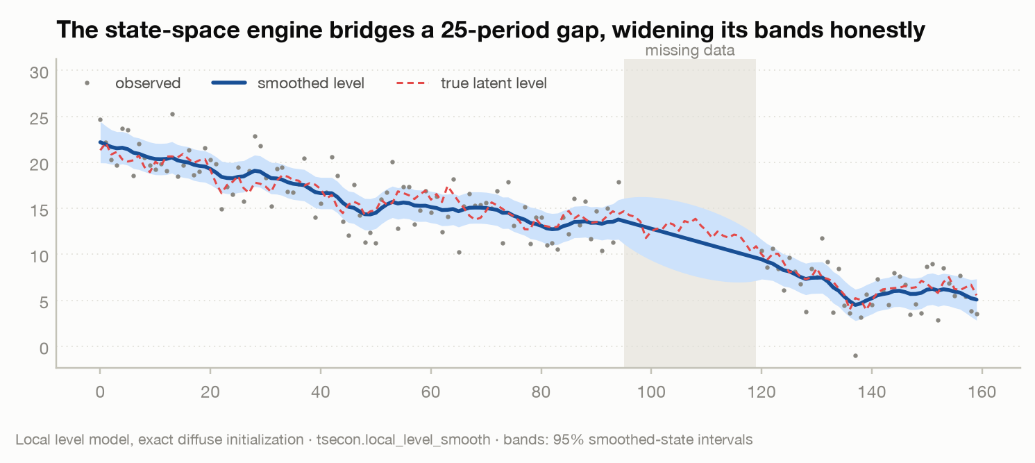
Read the figure as a miniature nowcast: inside the gap the smoother's estimate is the model's best guess given everything before and after, and the 95% band balloons to say so honestly. In a nowcasting DFM the same machinery runs over dozens of series at once, and "the gap" is the ragged edge at the bottom of the panel — the smoothed factor at the final month, projected through the triangle weights, is the GDP nowcast.
⚠ Common mistake — Zero-filling missing observations, or filling them with "a large measurement variance" as a hack. Both distort the likelihood; the second also destroys numerical precision (the related big-number trick for initializing the filter loses about seven digits exactly in mixed-frequency setups). The correct treatments are row selection or univariate filtering, and exact diffuse initialization — which is what the library's state-space core implements, and why it matches reference results at ~1e-11.
The two-step DFM nowcast in practice: dfm_nowcast
The section above demonstrated the load-bearing mechanism — a Kalman smoother bridging missing data — on a one-series local-level toy. Here is the panel version: dfm_nowcast runs the classic two-step dynamic-factor nowcaster of Doz, Giannone, and Reichlin (2011) over a whole ragged-edge panel, the estimator behind Giannone, Reichlin, and Small (2008).
"Two-step" names the estimation shortcut. Rather than the full EM iteration of Banbura and Modugno (2014), the two-step estimator does the cheap thing and it works: (1) extract the common factors and loadings by principal components on a balanced block of the panel; (2) fit a factor VAR of order \(p\) to those factors; then (3) plug the resulting state-space system into a single Kalman filter/smoother pass over the entire panel. Doz, Giannone, and Reichlin proved this two-step estimator is consistent as both dimensions grow, and it is an order of magnitude faster than EM — the reason it remains the workhorse for large-panel nowcasts where speed at each vintage matters.
The ragged edge is handled exactly as the conceptual section promised, and dfm_nowcast makes the division of labor explicit:
- Estimation runs on the balanced block. The two-step fit needs a complete rectangle to run PCA on, so the function takes the leading rows that are fully observed — every row before the first row containing any
NaN— as its training block. Publication lags live at the bottom of the panel, so this leading block is exactly the mature, fully-revised history. - Filtering runs on the full NaN-edge panel. With parameters in hand, the Kalman filter then sweeps the whole
T × Narray, and at each row uses exactly the cells that are present. The ragged staircase at the bottom — some series reporting the last month, others one or two months behind — is consumed as-is, no imputation.
The measurement equation for series \(i\) at the edge is just \(x_{i,t} = \lambda_i' f_t + e_{i,t}\), so once the filter has read the current-period factor \(f_t\) off whatever data did arrive, the missing cells are filled by projecting that factor back through the loadings. That projection is the nowcast. Here it is on a synthetic one-factor panel with the ragged edge punched into the last rows of two series:
import numpy as np
import tsecon

rng = np.random.default_rng(11)

# --- one latent factor with AR(2) dynamics drives a panel of N = 6 indicators ---
T, N = 150, 6
f = np.zeros(T)
for t in range(2, T):
    f[t] = 1.1 * f[t - 1] - 0.3 * f[t - 2] + rng.normal(scale=1.0)
load = np.array([1.0, 0.9, 0.8, 1.1, 0.7, 1.2])          # one loading per series
panel = f[:, None] * load[None, :] + rng.normal(scale=0.5, size=(T, N))

# --- the ragged edge: faster series are published further down the panel ---
panel[-1, 2] = np.nan          # series 2 has not released its last month
panel[-2:, 4] = np.nan         # series 4 is two months behind
print("last 3 rows (NaN = not yet released):")
print(np.round(panel[-3:], 2))

r = tsecon.dfm_nowcast(panel, n_factors=1, factor_order=2)
print("\nnowcast (filled edge, one level per series):", np.round(r["nowcast"], 2))
print("edge_factor:", np.round(r["edge_factor"], 3),
      " loglik:", round(r["loglik"], 1))

sf = np.asarray(r["smoothed_factors"])                    # over the balanced block
print("smoothed_factors shape:", sf.shape,
      " |corr| with true factor:",
      round(abs(np.corrcoef(sf[:, 0], f[:sf.shape[0]])[0, 1]), 3))
last 3 rows (NaN = not yet released):
[[-2.94 -1.42 -1.1  -1.82 -1.86 -3.4 ]
 [-2.13 -1.5  -0.94 -1.44   nan -1.75]
 [-1.32 -1.15   nan -1.56   nan -1.53]]

nowcast (filled edge, one level per series): [-1.36 -1.16 -1.01 -1.39 -0.91 -1.58]
edge_factor: [-1.985]  loglik: -438.5
smoothed_factors shape: (148, 1)  |corr| with true factor: 0.993
How to read the output. nowcast is the model's reconstruction of every series at the final period — one level per column. Two of those columns (nowcast[2] = -1.01 and nowcast[4] = -0.91) are genuine holes filled by the model, because series 2 and 4 had not reported their last months; the rest are the model-implied edge values for series that did report. Every entry is the corresponding loading times the shared edge_factor of \(-1.985\) (up to standardization and idiosyncratic noise), which is exactly the "smoothed factor at the final month, projected through the loadings, is the nowcast" statement from the section above, now concrete. The smoothed_factors array holds the full factor path over the balanced estimation block (148 rows here — the panel's 150 rows minus the two-row ragged tail); its near-perfect correlation with the simulated factor (\(0.993\)) confirms the two-step extraction recovered the latent driver. loglik is the Gaussian log-likelihood of the filtered panel, and n_factors / factor_order echo back the model dimensions for logging.
When to reach for it. dfm_nowcast is the right first tool for a genuine mixed-panel nowcast: a dozen-plus indicators, ragged edge, one shared cycle to read off. It supersedes running a separate bridge or MIDAS per indicator once the panel is wide, because it pools all the comovement into the factor and fills every hole from one estimated system. The "why did the nowcast move?" attribution does not require the elaborate machinery: dfm_news, the next section, runs the Banbura-Modugno decomposition off this same two-step fit. What is still roadmap is the full EM/block-DFM facade — Mariano-Murasawa quarterly-to-monthly aggregation, NY-Fed-style block loadings, EM under arbitrary missingness — which you want when missingness is heavy and interior rather than a tail edge; the two-step estimator is the fast, robust default that the more elaborate machinery is measured against.
⚠ Common mistake — Interspersing
NaNin the interior of the panel and expecting the two-step estimator to shrug it off. The training block is defined as the leading rows before the first row with any missing value, so a hole in the middle of an otherwise-complete series truncates the estimation sample to everything above it — silently throwing away data and, if the hole is early, leaving too few rows to fit the factor VAR. The two-step design assumes missingness lives at the ragged bottom edge (publication lags), which is the real-world case; genuinely interior gaps are the EM estimator's job. Also remember the factor's sign is not identified — a nowcast with the factor and all loadings flipped is the same model, which is why the diagnostic above takes the absolute correlation.
News decomposition: why did the nowcast move this morning?
A nowcast that moves without explanation is institutionally useless. The question every principal asks is not "what is the number?" but "why did it change since last week?" News decomposition — Banbura and Modugno (2014) — answers it exactly, and it is the feature that made the NY Fed's weekly nowcast publishable: each update comes with a bar chart attributing the revision to specific data releases.
The logic is clean. In a linear-Gaussian model with fixed parameters, the nowcast is a linear function of the data. When the information set grows from \(\Omega_v\) to \(\Omega_{v+1}\), only genuine surprises move the expectation:
where each weight \(b_j\) falls out of the Kalman smoother (it is the projection coefficient of the nowcast on release \(j\)'s innovation). A release that prints exactly at the model's expectation moves the nowcast by zero no matter how big the headline — only the unexpected component counts. The decomposition is additive and exact: the bars sum to the total revision.
A concrete reading. Suppose payrolls print at +250 thousand when the model expected +170: the news is +80. If the smoother-implied weight of that release on the GDP nowcast is 0.004 percentage points per thousand jobs, payrolls contributed \(0.004 \times 80 = +0.32\) points to this morning's revision. If industrial production simultaneously printed 0.3 below its expectation with a weight of 0.5, it contributed \(-0.15\). Net move: \(+0.17\), decomposed to the basis point — and the weight itself is diagnostic, telling you which releases the model actually listens to (survey data dominate early in the quarter, hard data late, a pattern the news weights make visible without any extra analysis).
Two subtleties keep this honest. If the model's parameters were re-estimated between the two dates, the identity above no longer holds exactly; the honest report includes a separate "parameter revision" remainder rather than smearing it across releases. And a revision to a previously published number is a different animal from a new release — a careful implementation attributes the two separately.
⚠ Common mistake — Computing "news" by re-running a re-estimated model and calling the whole difference in nowcasts the impact of the week's data. Part of that difference is parameter drift, not news. If the bars do not sum to the revision, or you cannot say which part is the remainder, the decomposition is decoration rather than accounting.
This is tsecon.dfm_news, and it takes the mistake box seriously: it fits the two-step DFM once, on the balanced block of the old vintage, and holds those parameters fixed across both vintages — so the identity above holds exactly and there is no parameter-drift remainder to smear. You hand it two panels of the same shape, the newer one revealing additional ragged-edge cells. Continuing the panel from the section above, suppose three more series have since printed their last month:
new_v = panel                      # this morning's vintage (as fitted above)
old_v = new_v.copy()               # last week's: three more cells still unreleased
old_v[-1, 0] = np.nan
old_v[-1, 1] = np.nan
old_v[-1, 3] = np.nan

nw = tsecon.dfm_news(old_v, new_v, target_series=4, n_factors=1, factor_order=2)
print("old nowcast:", round(nw["old_nowcast"], 3),
      " new:", round(nw["new_nowcast"], 3),
      " revision:", round(nw["total_revision"], 3))
for c in sorted(nw["contributions"], key=lambda c: -abs(c["contribution"])):
    print(f"  series {c['series']} @ t={c['period']}: "
          f"news {c['news']:+.3f} x weight {c['weight']:+.3f} = {c['contribution']:+.3f}")
print("bars sum to:", round(sum(c["contribution"] for c in nw["contributions"]), 6))
old nowcast: -0.849  new: -0.914  revision: -0.066
  series 3 @ t=149: news -0.265 x weight +0.159 = -0.042
  series 1 @ t=149: news -0.077 x weight +0.193 = -0.015
  series 0 @ t=149: news -0.051 x weight +0.176 = -0.009
bars sum to: -0.065677
Series 4 is the target because it is the genuine hole — two months behind, so its "nowcast" is entirely model-implied, the GDP-shaped case. Every row is the algebra of the display equation made literal: contribution = weight * news, the three bars sum to the total revision to the last digit printed, and the weights rank the releases by how much this model actually listens to them (series 3's larger loading buys it the largest weight, so its \(-0.265\) surprise does most of the work). A release that prints at expectation contributes zero regardless of its headline — that is the news column being zero, not the weight.
⚠ Common mistake — Passing non-nested vintages.
dfm_newsis a new-release decomposition, not a data-revision one: the new vintage must be a superset of the old, every previously observed cell still present and unchanged. It does not smear a revised past value across the bars — it refuses, withValueError: a cell observed in the old vintage is missing or changed in the new vintage. That is the second subtlety above enforced rather than documented; split the release effect from the revision effect yourself, in two calls.
Mixed-frequency VARs, briefly
The DFM compresses the panel into a few factors. A mixed-frequency VAR keeps every variable's own dynamics and cross-effects — the right tool when you care about the joint system (how GDP, inflation, and financial conditions interact) and not only the GDP nowcast. Two architectures dominate:
- Stacked (observation-driven) — Ghysels (2016): treat the \(m\) intra-quarter values of each monthly variable as \(m\) distinct elements of one quarterly vector, and run an ordinary VAR on the stacked system. No latent states, OLS-estimable, and it delivers impulse responses at mixed frequencies (how does a first-month shock differ from a third-month shock?). The cost is parameter proliferation as \(m\) and the lag count grow.
- State-space (parameter-driven) — Schorfheide and Song (2015): the VAR runs at the monthly frequency, and quarterly observables are linked to the monthly states through aggregation constraints, exactly as in the DFM's measurement equation. Estimation is Bayesian — a Gibbs sampler alternating a simulation smoother for the states with standard Minnesota-prior VAR posterior draws. This is the canonical central-bank formulation, and large versions of it nowcast about as well as DFMs (Cimadomo, Giannone, Lenza, Monti, and Sokol 2022).
Mixed-frequency VARs also repair a subtle inferential problem: testing Granger causality after aggregating everything to the lowest common frequency can manufacture causality that does not exist at the native frequency (and hide causality that does). Ghysels, Hill, and Motegi (2016) build causality tests directly on the stacked system to avoid the aggregation bias — a tool with essentially no maintained implementation in any language, which the roadmap carries for exactly that reason.
The library's roadmap carries both architectures, with the Schorfheide-Song sampler as the headline Bayesian model; single-frequency VAR machinery (var_fit, var_irf, and friends) is in the VAR chapter and available today.
⚠ Common mistake — Reading stacked MF-VAR impulse responses without checking the intra-period ordering convention. In the stacked system, "month 1", "month 2", and "month 3" of a quarter are different variables, and which within-quarter position a shock hits changes what the response means. The ordering is a modeling choice that must be stated, not a default to be discovered later.
Real-time evaluation: the discipline layer
Nothing in this chapter matters if the evaluation is dishonest, and nowcasting evaluations are dishonest in well-catalogued ways. A pseudo real-time exercise walks a nowcast origin through history: at each hypothetical date \(v\), reconstruct the information set \(\Omega_v\) (true vintages if you have them; otherwise today's data with the ragged edge simulated from publication lags), re-do everything — standardization, model selection, estimation — using only \(\Omega_v\), record the nowcast, and move on. Giannone, Reichlin, and Small (2008) set the pattern; Banbura, Giannone, Modugno, and Reichlin (2013) codified it. The signature output is not one RMSE but a curve: accuracy as a function of days-to-release, showing the nowcast sharpening as the quarter fills in.
Three rules carry most of the weight:
- No leakage. Anything fit on the full sample before the loop — a standardization, a factor extraction, a tuned hyperparameter, a variable selection — quietly hands the model future information.
- Declare your "actuals." Is truth the first release or the latest vintage? Model rankings flip with this choice, so it must be explicit, not defaulted.
- Use the right test. Most nowcast comparisons pit an indicator model against a nested benchmark (an AR or a mean), which invalidates the standard Diebold-Mariano test; Clark and West (2007) is the appropriate default there, and it ships as
tsecon.cw_test— one-sided, with the null that the small nested model is as good. Reach fordm_testonly when the two models are genuinely non-nested, as in the loop below.
A minimal pseudo real-time loop, with everything re-estimated inside each origin, runs today (continuing the bridge example's data). Written out by hand, because the point is to see rule 1 enforced line by line — tsecon.backtest drives the same expanding-window discipline for you and takes a Python callable, which is the shorter route once you trust the loop:
e_bridge, e_rw = [], []
for q in range(60, 80):                        # 20 pseudo real-time nowcast origins
    seen = x[:3 * q + 1]                       # first month of quarter q in hand
    fill = tsecon.theta_forecast(seen, steps=2)
    xq_now = np.r_[seen[-1:], fill].mean()
    X = np.column_stack([np.ones(q), xq[:q]])
    fit = tsecon.ols(gdp[:q], X, se_type="hac")    # re-estimated at every origin
    a, b = fit["params"]
    e_bridge.append(gdp[q] - (a + b * xq_now))
    e_rw.append(gdp[q] - gdp[q - 1])           # random-walk benchmark
e_bridge, e_rw = np.array(e_bridge), np.array(e_rw)

acc = tsecon.accuracy(gdp[60:], gdp[60:] - e_bridge, insample=gdp[:60])
dm = tsecon.dm_test(e_rw, e_bridge, h=1, loss="squared")
print(f"bridge MASE {acc['mase']:.2f},  DM (HLN) p-value {dm['p_value']:.3f}")
The bridge-versus-random-walk comparison here is non-nested, so Diebold-Mariano applies; had the benchmark been the bridge's own AR terms, it would not. Run it and you will see the other lesson live: the bridge posts a MASE below one, yet with only twenty origins the DM test cannot declare the difference significant — short, underpowered evaluation windows are the permanent condition of nowcast evaluation, which is why the field leans on fixed-b corrections and fluctuation tests rather than full-sample averages alone. The roadmap's evaluation harness automates the whole discipline — vintage reconstruction, in-loop refitting, the actuals declaration, Clark-West for nested pairs, and RMSE-by-days-to-release curves.
⚠ Common mistake — Standardizing the panel (or extracting factors, or selecting variables) on the full sample before the evaluation loop. This is the single most common bug in published nowcasting comparisons: every operation that looks at data must live inside the vintage loop. The symptom is a backtest that outperforms the same model run live — by the time you observe the symptom, the paper is usually already out.
Temporal disaggregation: Chow-Lin in brief
A cousin of nowcasting rather than the thing itself: sometimes you need a monthly path for a series that only exists quarterly (monthly GDP for a business-cycle chart, say). Temporal disaggregation distributes a low-frequency series across high-frequency periods using related indicators, under the hard constraint that the pieces aggregate back exactly.
Chow and Lin (1971) pose it as a GLS problem: assume a high-frequency regression \(y_t = X_t\beta + u_t\) with AR(1) errors, observe only the aggregated \(\tilde{y}_Q = C y\) (with \(C\) the aggregation matrix), estimate \(\beta\) and the AR parameter \(\rho\) from the aggregated model, and distribute the residual by its best linear unbiased prediction. Practical wrinkles the roadmap encodes: the \(\rho\) estimate routinely hits the unit boundary (detect it and fall back to Fernández's random-walk variant), and the Denton family — pure benchmarking without regressors — should default to the Denton-Cholette variant, which fixes a known artifact in the original's first periods. In state-space form (Proietti 2006, via "cumulator" states) all of this falls out of the same Kalman machinery as the rest of the chapter, ragged edges and extrapolation included.
⚠ Common mistake — Interpolating a quarterly series with a spline or a naive regression and then rescaling the months so they add up. Post-hoc rescaling distorts the within-quarter profile in exactly the periods where it matters most. The BLUE distribution formula satisfies the aggregation constraint by construction; if your disaggregated series needs a correction step at the end, the method upstream is wrong.
The frontier
The research edge of nowcasting is mostly about making the core architecture honest in hard conditions:
- Pandemic-scale outliers. 2020Q2 was roughly a fifteen-sigma observation; Gaussian EM estimates simply break. The fixes — Student-t idiosyncratic errors, explicit outlier states, volatility rescaling — are now effectively mandatory equipment (Antolin-Diaz, Drechsel, and Petrella 2024; Lenza and Primiceri 2022; Schorfheide and Song 2024 for the MF-VAR analog). A library that silently Gaussian-fits 2020 produces garbage factors without an error message, which is why the roadmap treats outlier detection with loud warnings as default behavior.
- Drifting trend growth and stochastic volatility. Antolin-Diaz, Drechsel, and Petrella (2017) showed that letting long-run growth drift materially improves nowcasts (and avoids systematic bias when trend growth slows); stochastic volatility does the same for density nowcasts.
- Higher frequency. Weekly and daily activity indexes — the Aruoba-Diebold-Scotti index (2009) and the Weekly Economic Index (Lewis, Mertens, Stock, and Trivedi 2022) — push the same state-space architecture to frequencies where the calendar itself (52/53-week years, trading days) becomes the hard engineering problem.
- High-dimensional and ML nowcasting. The sg-LASSO MIDAS of Babii, Ghysels, and Striaukas (2022) handles hundreds of daily predictors with structured sparsity; tree ensembles and neural nets are competitive in nonlinear episodes but demand the same vintage discipline, and interpretability is the open front — there is no accepted analog of Kalman news decomposition for ML nowcasts (Shapley-value attributions over release sets are the emerging candidate).
- Distributional nowcasting. Growth-at-Risk — nowcasting the tails, not the mean, of the GDP distribution (Adams, Adrian, Boyarchenko, and Giannone 2021) — via quantile MIDAS and quantile factor models. The single-frequency half of this is behind you already:
growth_at_riskfits the Adrian-Boyarchenko-Giannone conditional quantiles at every observation, with the Chernozhukov-Fernández-Val-Galichon rearrangement and a crossing report (Chapter 5), andquantile_lpgives the dynamic version (Chapter 9). The mixed-frequency members — quantile MIDAS, quantile factor models — are the frontier part.
The library's roadmap (Module 08) treats this whole stack as its headline differentiator, and the first courses are laid: dfm_nowcast, dfm_news, umidas and weighted_midas ship, so the panel nowcast and its release attribution are callable today. What still has no maintained home in Python — tsecon's included — is the end-to-end system around them: statsmodels 0.15 gives you DynamicFactorMQ (with a news() method of its own) but no vintage store, no release calendar, and no pseudo-real-time harness wired to either, and every central-bank shop rebuilds that plumbing from scratch. The stated validation bar for the rest is concrete: reproduce the NY Fed replication code's nowcast paths to three-plus decimals, match DynamicFactorMQ likelihoods and news() output, match the Schorfheide-Song replication and R's midasr coefficient-for-coefficient — and beat the reference implementations on speed by an order of magnitude. What ships today is graded more modestly and says so: dfm_nowcast's Kalman step is pinned against statsmodels DynamicFactor at fixed parameters (the two-step estimates are property-tested, not reference-matched), and dfm_news against an independent NumPy Kalman/RTS implementation of Banbura-Modugno. Honest open problems remain: news-vs-noise revision modeling is fragile to identify (Jacobs and van Norden 2011), evaluation windows are short enough that test power is a real constraint, and alternative-data indicators are silently revised in ways that invalidate naive backtests.
Which method when
| Situation | Reach for | Because |
|---|---|---|
| A few monthly indicators, need something defensible this week | Bridge equations by hand — theta_forecast to complete the indicator, ols(se_type="hac") for the bridge — pooled across indicators |
Transparent, robust, and pooling beats picking a winner (Kuzin et al. 2013) |
| Monthly indicators, quarterly target (\(m = 3\)) | umidas |
With few lags, unrestricted OLS dominates restricted weights (Foroni et al. 2015) |
| Daily/weekly indicators, quarterly target (\(m\) large) | weighted_midas with scheme="exp_almon" or "beta" |
Hundreds of lags need a parsimonious weight curve to avoid parameter explosion |
| Persistent target, want dynamics done right | adl_midas (ADL-MIDAS: umidas plus ar_lags lags of the target, HAC bandwidth on the rows actually fitted) |
AR terms are not optional for macro series; plain MIDAS is a straw man |
| Mid-quarter update using this quarter's own months | MIDAS with leads, calendar-driven — roadmap (the library ships no release calendar) | Within-quarter data are the point of nowcasting; the calendar prevents off-by-one leaks |
| Large mixed panel, ragged edge, institutional nowcast | dfm_nowcast(panel, n_factors, factor_order) |
Kalman filter consumes the staircase natively; one model, whole panel |
| "Why did the nowcast move today?" | dfm_news(old_vintage, new_vintage) |
Exact, additive attribution of revisions to releases (Banbura-Modugno 2014); the bars sum to the revision |
| Joint dynamics and density nowcasts across frequencies | MF-VAR (Schorfheide-Song) — roadmap; var_fit and friends cover the single-frequency case |
Keeps every variable's dynamics; Bayesian shrinkage handles the dimension |
| Need a monthly path for a quarterly-only series | Chow-Lin / Denton-Cholette disaggregation — roadmap | Constraint-exact distribution, not an ad hoc interpolation |
| Claiming your model beats the benchmark | backtest (it takes a Python callable, so your nowcast function goes straight in), then cw_test |
Revised-data backtests flatter you; nested comparisons invalidate plain DM, which is what cw_test repairs |
What tsecon implements today
Available now in Python (import tsecon):
dfm_nowcast(data, n_factors, factor_order, method="two_step"|"mle")— the Doz-Giannone-Reichlin two-step dynamic-factor nowcaster over a ragged-edge panel (or the one-step MLE route), returning the edgenowcast, theedge_factor,smoothed_factors, and the full reproducible parameter surface (loadings,factor_ar,factor_cov,idiosyncratic,center,scale)dfm_news(old_vintage, new_vintage, target_series=…)— the Banbura-Modugno revision decomposition off that same fit: per-datapoint{series, period, actual, forecast, news, weight, contribution}whose contributions sum exactly tototal_revisionumidas(y, hf_lags, se_type="hac")andweighted_midas(y, hf_lags, scheme="exp_almon"|"beta")— unrestricted MIDAS by OLS and the two-parameter restricted-weight fit by NLS, withmidas_weights(scheme, theta1, theta2, k)for the weight curve itselflocal_level_smooth(y, sigma2_eps, sigma2_eta)— the exact-diffuse Kalman filter/smoother with native NaN handling: the core mechanism of every state-space nowcaster, demonstrated above bridging a 25-period gapar_loglik(y, coeffs, sigma2, intercept)— the exact state-space likelihood kernelols(y, X, se_type="hac")— bridge equations and hand-rolled Almon-MIDAS via the design-matrix transform, with honest standard errorstheta_forecast(y, steps, period)— indicator completion for bridge equationsbacktest(y, forecaster=…)— the rolling/expanding pseudo-out-of-sample engine, which accepts a plain Python callable, so a whole nowcast pipeline can be graded under its leakage disciplineaccuracy(actual, forecast, insample=...),dm_test(e1, e2, h, loss),cw_test(...)— the evaluation layer for pseudo real-time loops, Clark-West included for the nested comparisons that plain DM cannot handlevar_fit,var_forecast,var_irf,var_fevd,var_granger— single-frequency VAR machineryhp_filter(y, one_sided=True)— the real-time (one-sided) trend variant, relevant whenever a "current trend" enters a nowcast
Built in Rust, awaiting Python bindings: the general linear-Gaussian state-space engine behind local_level_smooth (the tsecon-ssm crate) — arbitrary state-space models, exact diffuse initialization, filtering and smoothing with missing data handled by construction. This is the foundation the entire nowcasting stack builds on.
Roadmap (Module 08 — Nowcasting and Mixed Frequency): the release-calendar and vintage layer, bridge-equation suites with pooling, the rest of the MIDAS family (leads, Bayesian and quantile variants — the unrestricted, autoregressive, exponential-Almon and beta members ship as umidas/adl_midas/weighted_midas), the EM/block-loading DFM facade for heavy interior missingness (the two-step nowcast and its news decomposition ship as dfm_nowcast/dfm_news, and dfm_smooth re-smooths a new vintage at a fitted model's parameters), Schorfheide-Song and stacked MF-VARs, Chow-Lin/Denton-Cholette temporal disaggregation, and the leakage-proof pseudo real-time evaluation harness — the general-purpose backtest engine covers the single-series case today, but nothing yet automates vintage replay.
Further reading
- Giannone, Reichlin & Small (2008, Journal of Monetary Economics) — the paper that coined "nowcasting" and set the DFM-plus-real-time-evaluation template everyone still follows.
- Banbura & Modugno (2014, Journal of Applied Econometrics) — EM estimation under arbitrary missing data and the exact news decomposition; the two pillars of the modern nowcasting DFM.
- Banbura, Giannone, Modugno & Reichlin (2013, Handbook of Economic Forecasting) — the canonical survey of nowcasting theory and practice.
- Bok, Caratelli, Giannone, Sbordone & Tambalotti (2018, Annual Review of Economics) — the NY Fed Nowcast, documented end to end; the architecture this chapter calls "the flagship".
- Ghysels, Santa-Clara & Valkanov (2005, Journal of Financial Economics) — the founding MIDAS application; the 2004 working paper introduced the framework.
- Foroni, Marcellino & Schumacher (2015, Journal of the Royal Statistical Society, Series A) — U-MIDAS, and the honest answer to when weight restrictions help versus hurt.
- Schorfheide & Song (2015, Journal of Business & Economic Statistics) — the canonical Bayesian mixed-frequency VAR.
- Mariano & Murasawa (2003, Journal of Applied Econometrics) — the triangle aggregation linking quarterly observables to monthly states; five weights that appear in every mixed-frequency measurement equation.
- Croushore & Stark (2001, Journal of Econometrics) — the real-time dataset: why vintages exist as a research object and why revised-data results mislead.
- Chow & Lin (1971, Review of Economics and Statistics) — temporal disaggregation as GLS; still the default answer fifty years on.
- Durbin & Koopman, Time Series Analysis by State Space Methods (2012, 2nd ed.) — the textbook for the Kalman machinery under all of this: missing data, diffuse initialization, smoothing.