Model card — ARIMA

arima_fit · ar_loglik

ARIMA is the flagship classical univariate model: the endpoint of the AR → MA → ARMA → ARIMA ladder that turns two simple ideas — the past predicts the future (autoregression) and past surprises linger (moving average) — into one forecasting workhorse. The recipe is "difference d times to reach stationarity, then fit an ARMA(p,q)":

phi(L) (1 - L)^d y_t = c + theta(L) eps_t,        eps_t ~ iid N(0, sigma^2)

where phi(L) = 1 - phi_1 L - ... - phi_p L^p is the autoregressive polynomial, theta(L) = 1 + theta_1 L + ... + theta_q L^q the moving-average polynomial, and (1 - L) y_t = y_t - y_{t-1} the first difference. This card covers the full exact-MLE estimator (arima_fit) and the fixed-parameter AR log-likelihood helper (ar_loglik) that exposes the same likelihood kernel as a scoring function. Both run on one state-space engine: the Harvey canonical form of the ARMA process evaluated by the Kalman filter's prediction-error decomposition — the same machinery that underlies local_level_smooth and the module's exact-diffuse Kalman work. For end-to-end forecasting, evaluation, and benchmarking, pair this card with the Forecasting card.

---

arima_fit — exact-MLE ARIMA(p,d,q) fit and forecast

What it estimates. The parameters of an ARIMA(p,d,q) model by exact maximum likelihood — the AR coefficients phi_1..phi_p, the MA coefficients theta_1..theta_q, an optional constant c, and the innovation variance sigma^2 — together with the log-likelihood, AIC/BIC, the one-step residuals, and (optionally) multi-step point forecasts with prediction intervals that are correctly integrated back to the original scale. Estimation differences the series d times, maximizes the exact Gaussian likelihood of the differenced ARMA process via the Kalman filter's prediction-error decomposition, and undifferences the forecasts so their variance compounds across the integration.

Assumptions. After d differences the series is covariance-stationary and invertible; the innovations are Gaussian white noise (the likelihood is exact under Gaussianity and quasi-ML otherwise); the AR roots lie outside the unit circle and the MA roots outside or on it. d is a modeling decision you make before fitting — with unit-root tests, not an information criterion — because likelihoods computed at different d are likelihoods of different datasets and are not comparable. The exact likelihood additionally treats the initial observations as draws from the process's own stationary distribution, which is exactly the information CSS throws away and where the two estimators diverge in small samples and near the unit circle.

When to use (and when not). Use it as the default forecast for a single series with momentum: difference a trending level (GDP, prices, the money stock) to stationarity with d = 1 (rarely d = 2), capture short-run dynamics with a small number of AR and MA terms, and read off point forecasts with honest widening intervals. Prefer exact MLE over CSS or Yule-Walker whenever the sample is short or persistence sits near a unit root — the initial conditions carry real information and moment methods bias toward stationarity. Do not let AIC pick d (choose it with check_stationarity); do not overfit ARMA orders — an ARMA(2,2) on ARMA(1,1) data creates near-canceling AR/MA roots, a flat likelihood, and fragile estimates with huge standard errors; do not difference through missing values (fit in levels via the state-space form instead); and do not reach here for seasonal structure — the SARIMA (P,D,Q,s) layer is not yet in this estimator (it is on the Module 02 roadmap).

Key arguments and defaults (and why). p, d, q are the orders (all default 0). constant = False — a mean/drift term is off by default because for a differenced (d >= 1) series a constant is a deterministic drift, which you should add deliberately, not by accident; for d = 0 it is the level term, and note the fitted const is c, not the process mean, which is c / (1 - sum phi). forecast_steps = 0 — set it to the horizon h to return h-step forecasts. conf_alpha = None — leave it None for point forecasts and standard errors only; set it (e.g. 0.05 for 95%) to also return symmetric Gaussian prediction bands. conf_alpha requires forecast_steps > 0 and must lie in (0, 1); both are validated (a ValueError, not a silent default). Under the hood the optimizer uses Hannan-Rissanen (1982) starting values and the Monahan (1984) reparameterization to keep the search inside the stationary-and-invertible region (whose admissible set for p, q > 1 is not a box, so naive coefficient bounds fail) — you do not tune these, but they are why the fit is robust.

How to read the output. A dict. params is the coefficient vector in the order named by param_names — ["const"?, "ar.L1"..., "ma.L1"..., "sigma2"] (the constant appears only when constant=True, and sigma2 is always last and is counted as a free parameter in the ICs, matching statsmodels). loglik is the maximized exact log-likelihood; aic and bic are -2 loglik + 2k and -2 loglik + k log T. residuals are the one-step-ahead innovations (feed them to ljung_box — remembering to dock the degrees of freedom by p + q — and to arch_lm). When forecast_steps > 0: forecast_mean and forecast_se are the h-step point forecasts and their standard errors on the original (undifferenced) scale, forecast_se widening monotonically with the horizon. When conf_alpha is set, forecast_lower/forecast_upper are mean ± z(alpha) * se and conf_alpha echoes the coverage you asked for.

Failure modes. Overdifferencing injects an MA unit root (theta ≈ -1, the likelihood piling on the invertibility boundary, first-lag autocorrelation of the difference near -0.5) — the symptom of differencing an already-stationary series. Overfit orders produce near-canceling roots and offsetting AR/MA coefficients with inflated standard errors — shrink the model when you see them. Comparing this log-likelihood to another package's without matching conventions (the Gaussian constant, diffuse-term handling, whether sigma2 is concentrated out) manufactures phantom disagreements; a gap of exactly (T/2) log 2pi is a convention, not a bug. Passing a series with NaNs, or one too short for the requested orders, raises rather than guessing. And prediction intervals are Gaussian and condition on the fitted parameters — they ignore parameter and model-selection uncertainty and so are, like everyone's, somewhat too narrow near unit roots and for T < 100.

Validated against. statsmodels 0.14.6 SARIMAX, on documented fixtures (fixtures/arima.json) and live tests. The Rust golden pins fixed-parameter exact log-likelihoods to 1e-8 relative — ARMA(1,1) demeaned against SARIMAX(order=(1,0,1)).loglike, and ARIMA(1,1,1) with simple differencing on the Nile against SARIMAX(order=(1,1,1), simple_differencing=True).loglike. For the full exact-MLE fit of ARMA(1,1)+constant on the Nile the estimator is held to a match-or-beat floor on the log-likelihood and to 1e-4 relative on the parameters against an independently cross-verified maximizer. That gate has a story worth telling: statsmodels' default fit stalls at loglik = -638.117 (a point where its own numerical gradient is O(1e-2)), while tsecon reaches the genuine optimum at loglik = -637.039 — a better fit than the reference, confirmed by re-optimizing statsmodels' own objective from its stopping point. The Python side (test_smoke.py::test_arima_fit_beats_statsmodels_on_nile, test_arima_d1_random_walk_law, and the test_intervals.py interval round-trips) asserts the beat, the monotone forecast SE, white-noise residuals, and the exact se_h = sigma * sqrt(h) law for a random walk.

References. Box & Jenkins (1970, Time Series Analysis: Forecasting and Control, Holden-Day); Harvey (1989, Forecasting, Structural Time Series Models and the Kalman Filter, CUP, §3.3–3.4, the state-space form and prediction-error decomposition); Hannan & Rissanen (1982, Biometrika 69:81–94, starting values); Monahan (1984, Biometrika 71:403–404, the stationary/invertible reparameterization); Durbin & Koopman (2012, Time Series Analysis by State Space Methods, 2nd ed., OUP).

import numpy as np, tsecon

# --- A synthetic stationary ARMA(1,1): mean 4, phi = 0.6, theta = 0.3 ---
rng = np.random.default_rng(11)
n, phi, theta, mu = 500, 0.6, 0.3, 4.0
eps = rng.standard_normal(n)
y = np.empty(n); y[0] = mu + eps[0]; e_prev = eps[0]
for t in range(1, n):
    y[t] = mu + phi * (y[t - 1] - mu) + eps[t] + theta * e_prev
    e_prev = eps[t]

fit = tsecon.arima_fit(y, p=1, d=0, q=1, constant=True,
                       forecast_steps=8, conf_alpha=0.05)
names = list(fit["param_names"])
for nm, v in zip(names, fit["params"]):
    print(f"{nm:8s} = {v:+.4f}")
print(f"loglik = {fit['loglik']:.2f}   AIC = {fit['aic']:.1f}   BIC = {fit['bic']:.1f}")
c, ar1 = fit["params"][names.index("const")], fit["params"][names.index("ar.L1")]
print(f"implied mean  c/(1-phi) = {c / (1 - ar1):.3f}")   # NOT the intercept itself
print(f"Ljung-Box(10) p-value   = "
      f"{tsecon.ljung_box(fit['residuals'], nlags=10)['lb_pvalue'][-1]:.3f}")
print("forecast_mean:", np.round(fit["forecast_mean"], 3))
print("forecast_se  :", np.round(fit["forecast_se"], 3))
print(f"95% band, step 1: [{fit['forecast_lower'][0]:.2f}, {fit['forecast_upper'][0]:.2f}]")
# const    = +1.9949
# ar.L1    = +0.5134
# ma.L1    = +0.3649
# sigma2   = +0.9343
# loglik = -692.87   AIC = 1393.7   BIC = 1410.6
# implied mean  c/(1-phi) = 4.100
# Ljung-Box(10) p-value   = 0.583
# forecast_mean: [4.227 4.165 4.133 4.117 4.109 4.104 4.102 4.101]
# forecast_se  : [0.967 1.286 1.358 1.377 1.381 1.383 1.383 1.383]
# 95% band, step 1: [2.33, 6.12]

The fitted const (1.995) is not the mean — the mean is c / (1 - phi) = 4.10, recovering the true 4.0. The intervals widen monotonically toward the unconditional variance, which is exactly the fan chart the gallery draws:

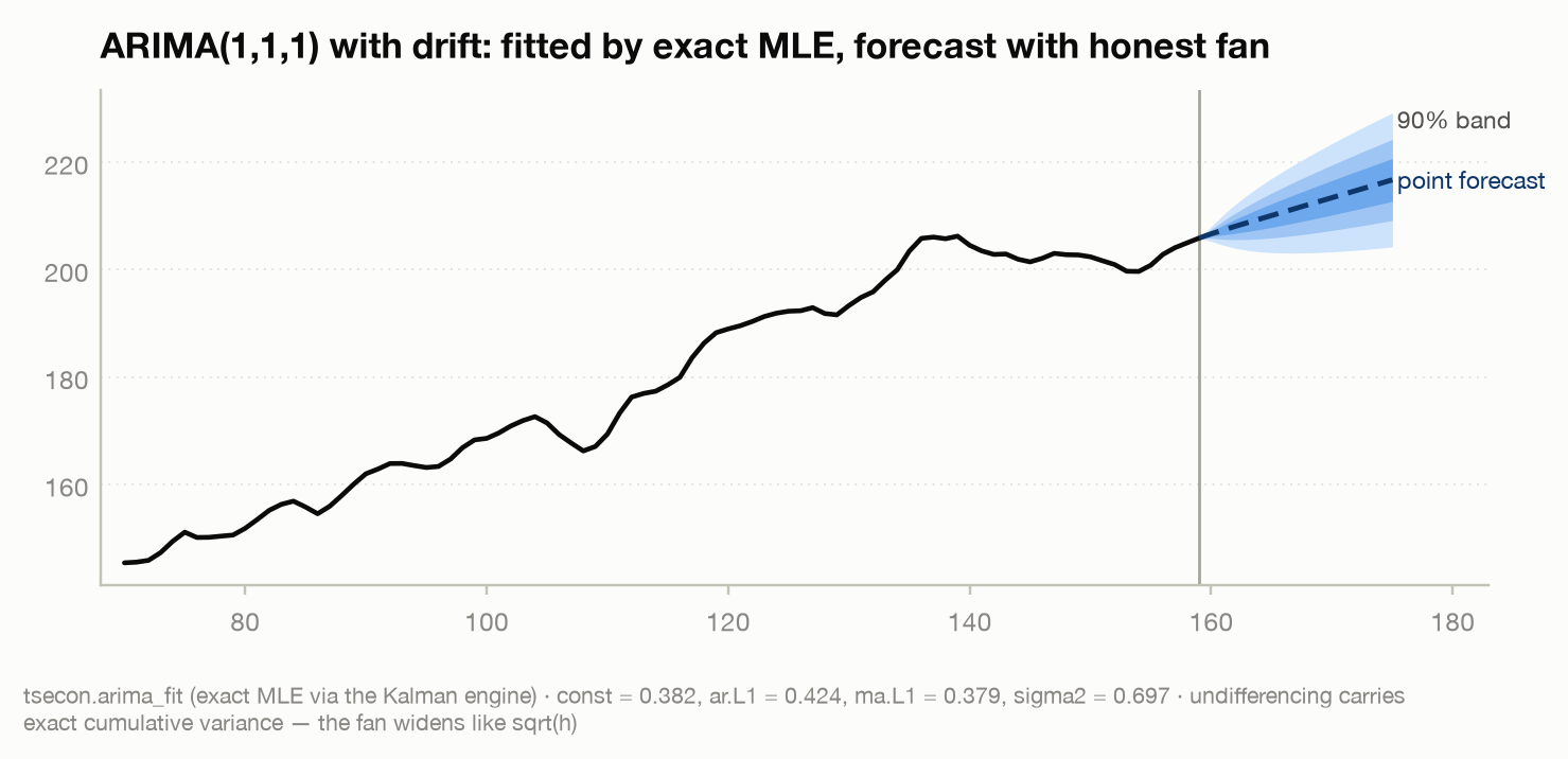
The √h law, made visible. For a pure random walk (p=0, d=1, q=0, no constant) ARIMA theory says the forecast standard error must grow as sigma * sqrt(h) — the variance of a sum of h independent innovations. The integrated-back intervals reproduce it to machine precision:

import numpy as np, tsecon

rng = np.random.default_rng(3)
rw = np.cumsum(rng.standard_normal(400)) * 1.7      # a pure random walk, I(1)
r = tsecon.arima_fit(rw, p=0, d=1, q=0, constant=False, forecast_steps=6)
print("forecast_se        :", np.round(r["forecast_se"], 4))
ratio = r["forecast_se"] / (r["forecast_se"][0] * np.sqrt(np.arange(1, 7)))
print("se_h / (se_1*sqrt h):", np.round(ratio, 8))
# forecast_se        : [1.7078 2.4152 2.958  3.4156 3.8187 4.1832]
# se_h / (se_1*sqrt h): [1. 1. 1. 1. 1. 1.]

---

ar_loglik — exact AR(p) log-likelihood at fixed parameters

What it estimates. Nothing — it evaluates. Given a series and a fixed AR(p) parameter vector, it returns the exact Gaussian log-likelihood of an AR(p) model with optional intercept, computed via the same state-space form and stationary initialization as the full ARIMA fit (and matching statsmodels SARIMAX(trend='c') conventions). It is the scoring kernel the exact-MLE estimator maximizes, exposed directly: a single number you can grid, profile, or hand to your own optimizer.

Assumptions. The series is a stationary AR(p) with the supplied coefficients; the innovations are Gaussian white noise with the supplied variance. Because the initialization is the process's stationary distribution, the supplied coefficients must define a stationary AR — the admissible region is the AR stationarity simplex, not a coefficient box (for an AR(2), phi_1 + phi_2 < 1, phi_2 - phi_1 < 1, |phi_2| < 1), and the function refuses to evaluate outside it rather than returning a meaningless number.

When to use (and when not). Use it to see the likelihood machinery move: to score a candidate parameterization, to build a brute-force or profile MLE for teaching or diagnostics, to compare the evidence for a persistent versus a moderate model on a short stretch of data (the gap between two ar_loglik values includes the information in the initial observations that CSS discards), or as a fast, dependency-free likelihood inside a larger routine. Do not use it as a fitter — for a real fit call arima_fit, which optimizes this same likelihood with proper starting values and returns standard errors, ICs, and forecasts. It has no MA terms and no differencing: it is AR(p) in levels only.

Key arguments and defaults. y the series; coeffs the length-p AR vector [phi_1, ..., phi_p]; sigma2 the innovation variance (> 0); intercept = 0.0 the constant term c in y_t = c + sum phi_j y_{t-j} + eps_t — note again that c is not the mean, which is c / (1 - sum phi).

How to read the output. A single float: the exact Gaussian log-likelihood. Larger (less negative) is a better-fitting parameterization on the same data. Differences are the currency — the maximizer over a grid is an exact MLE of whatever you varied.

Failure modes. Passing non-stationary coefficients raises a ValueError (this is a guard, not a bug — the stationary initialization is undefined there). A non-positive sigma2 is rejected. Comparing ar_loglik values across different data, different p, or against another package's AR likelihood without matching the intercept/constant and Gaussian-constant conventions compares incomparable numbers.

Validated against. statsmodels SARIMAX. The live test (test_smoke.py::test_ar_loglik_matches_sarimax) pins the AR(2)-with-constant exact log-likelihood to 1e-9 relative against SARIMAX(order=(2,0,0), trend='c').loglike at the same fixed parameters — the tightest tolerance in the module, reflecting that this is the exact analytic likelihood, not an approximation.

References. Harvey (1989, §3.3–3.4); Durbin & Koopman (2012); the AR log-likelihood via the prediction-error decomposition is standard (e.g. Hamilton, 1994, Time Series Analysis, Princeton, ch. 5).

import numpy as np, tsecon

rng = np.random.default_rng(42)
n = 400
phi1, phi2 = 1.3, -0.4                       # a stationary AR(2)
y = np.zeros(n); eps = rng.standard_normal(n)
for t in range(2, n):
    y[t] = phi1 * y[t - 1] + phi2 * y[t - 2] + eps[t]

# The exact likelihood scores candidate parameters; the truth wins.
print(f"ar_loglik at truth  [ 1.3, -0.4] = {tsecon.ar_loglik(y, [1.3, -0.4], 1.0):.2f}")
print(f"ar_loglik at wrong  [ 0.9,  0.0] = {tsecon.ar_loglik(y, [0.9,  0.0], 1.0):.2f}")

# A brute-force 1-D exact MLE: profile phi1 with phi2 = -0.4 fixed.
grid = np.linspace(1.0, 1.39, 79)            # stationarity => phi1 + phi2 < 1
ll = [tsecon.ar_loglik(y, [g, -0.4], 1.0) for g in grid]
print(f"argmax phi1 (truth 1.3)          = {grid[int(np.argmax(ll))]:.4f}")

# The stationarity simplex is enforced, not a coefficient box.
try:
    tsecon.ar_loglik(y, [1.5, -0.4], 1.0)    # phi1 + phi2 = 1.1 > 1: non-stationary
except ValueError:
    print("non-stationary [1.5, -0.4]       -> ValueError (refused)")
# ar_loglik at truth  [ 1.3, -0.4] = -549.10
# ar_loglik at wrong  [ 0.9,  0.0] = -599.03
# argmax phi1 (truth 1.3)          = 1.2750
# non-stationary [1.5, -0.4]       -> ValueError (refused)

The profile lands near the true phi_1 = 1.3 (the coarse 79-point grid resolves to 1.275), and the truth out-scores the wrong model by ~50 log-likelihood units — the exact-MLE kernel arima_fit maximizes, laid bare.

---

See also the univariate models guide chapter for the full AR → MA → ARMA → ARIMA → SARIMA ladder and the CSS-versus-exact-MLE discussion, and the Forecasting card for backtesting and forecast-comparison tests to evaluate an ARIMA against benchmarks.