Chapter 5 — Forecasting: Practice and Evaluation
Part of The tsecon Guide to Time Series Econometrics. Chapters mirror the library's modules; code runs against the current Python API unless marked otherwise.
Prerequisites: OLS regression and standard errors, plus the stationarity and autocorrelation ideas from the earlier chapters; comfort with numpy arrays.
You will learn:
- What a forecast actually claims — and why a point forecast, an interval, and a full density are three different promises.
- Why in-sample fit is a lie, and how pseudo-out-of-sample backtesting with rolling or expanding origins replaces it.
- Why naive benchmarks are scandalously hard to beat, and what fifty years of forecasting competitions proved.
- How to score forecasts without fooling yourself — MAPE's failure modes, why MASE exists, and what pinball loss and CRPS measure.
- How to test whether an accuracy difference is real (Diebold-Mariano with the HLN correction), when that test is invalid, and what to run instead —
cw_testfor nested models,gw_testfor forecasting methods — and why averaging forecasts usually beats picking one. - How to put an honest interval around a point forecast without assuming a distribution — split conformal, ACI, and EnbPI — and how to grade the interval you get.
- Growth-at-risk: why policy institutions forecast the downside of the growth distribution, and how financial conditions move the left tail more than the center.
The idea
Suppose your model says inflation will be 2.4 percent next year. Should anyone believe you?
That question — not model estimation — is what forecasting practice is about. Producing a number is easy; every model in this guide will happily emit one. The hard discipline is measurement: how do you find out whether your forecasts are any good, whether they are better than an embarrassingly simple alternative, and whether an apparent improvement is real or a fluke of the particular years you tested on?
The central trap is that a model always looks best on the data it was fit to. Add lags, add predictors, add flexibility, and the in-sample errors shrink every time — that is arithmetic, not skill. The model is partly memorizing the noise in your sample, and noise does not repeat. So forecasters simulate the real situation instead: stand at some past date, fit the model using only data available then, forecast forward, and compare against what actually happened. Slide that origin date through history and you accumulate a track record of honest errors — a backtest. Everything else in this chapter is machinery built on that one picture: a vertical line sweeping left to right through your data, with the model repeatedly blindfolded to everything on the right of it.
The second trap is forecasting without a benchmark. The dumbest possible forecast — "tomorrow will be like today" — is, for many economic series, close to unbeatable. Exchange rates, stock returns, and (in some eras) inflation have humiliated generations of sophisticated models this way. A forecast error of 1.2 percentage points means nothing on its own; what matters is whether the no-thought benchmark scored 1.1. Never report a forecast without a benchmark, and never claim superiority without a test. That sentence is the whole chapter; the rest is how to do it properly.
What a forecast claims: point, interval, density
A practitioner cares because these three objects answer different questions, and mixing them up produces real damage — a budget office that treats a central GDP projection as a certainty has no plan for the recession scenario that the same model assigned 20 percent probability.
Behind every forecast is a predictive distribution: given everything known at time \(t\), the random variable \(y_{t+h}\) has some conditional distribution \(F_{t+h|t}\). The three kinds of forecast are three summaries of it:
- A point forecast \(\hat{y}_{t+h|t}\) is a single number — one functional of \(F_{t+h|t}\). Which functional is not a matter of taste: the point forecast that minimizes expected squared error is the conditional mean, while the one that minimizes expected absolute error is the conditional median (Gneiting 2011). A point forecast is only well-defined once you say which loss it is optimal for.
- An interval forecast \([l_{t+h|t},\, u_{t+h|t}]\) claims coverage: the realization should land inside with probability \(1-\alpha\),
- A density forecast hands over \(F_{t+h|t}\) itself — the whole distribution, usually as a set of quantiles or simulation draws. Central banks publish these as fan charts: nested shaded bands, one per coverage level, widening with horizon.
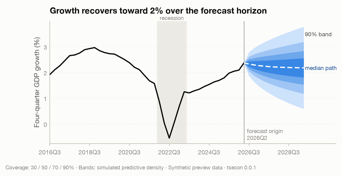
The fan chart above is the library's house rendering of a density forecast: the darkest ribbon is the central band, each lighter ribbon adds coverage, and the widening fan is the honest admission that uncertainty grows with horizon.
In tsecon today, var_forecast produces point forecasts with interval bands from a vector autoregression:
import numpy as np
import tsecon

rng = np.random.default_rng(42)
n = 240                                # two-variable system: "growth" and a leading "spread"
data = np.zeros((n, 2))
for t in range(1, n):
    data[t, 1] = 0.7 * data[t - 1, 1] + 0.5 * rng.standard_normal()
    data[t, 0] = 0.5 * data[t - 1, 0] + 0.3 * data[t - 1, 1] + 0.8 * rng.standard_normal()

fc = tsecon.var_forecast(data, lags=1, steps=8, alpha=0.05)
fc["point"]        # 8 x 2 central path
fc["lower"]        # 8 x 2 lower 95% band — widens with horizon
fc["upper"]
⚠ Common mistake. Reading pointwise interval bands as a statement about the whole path. The 95% band at each horizon says the realization at that horizon lands inside with 95% probability; the probability that the entire 8-step path stays inside all eight bands is well below 95%. Joint path bands are wider (Jordà and Marcellino 2010) and are a roadmap item.
One step ahead or many: iterated vs direct
Multi-step forecasts can be built two ways, and the choice changes both accuracy and the statistics you are allowed to use afterward.
The iterated (or recursive) strategy fits a one-step model and feeds its own forecasts back in: forecast \(t+1\), pretend it happened, forecast \(t+2\), and so on. This is what var_forecast does internally. The direct strategy fits a separate regression for each horizon, projecting \(y_{t+h}\) straight onto information at \(t\):
where \(x_t\) collects the predictors known at \(t\) and each horizon gets its own \(\beta_h\). Marcellino, Stock and Watson (2006) ran the horse race across 170 US monthly series: iterated forecasts usually win when the one-step model is well specified, because they use the data more efficiently; direct forecasts are more robust when the model is misspecified, because each horizon's errors are minimized directly rather than compounded through a wrong recursion.
The statistical fine print: a direct \(h\)-step regression has overlapping forecast errors. Even if the one-step-ahead world is unpredictable white noise, \(u_{t+h}\) is a moving average of order \(h-1\) by construction — consecutive errors share \(h-1\) of the same underlying shocks. Ordinary standard errors are therefore wrong, and you need the HAC machinery from the regression chapter with bandwidth at least \(h-1\):
h = 4                                   # direct 4-step projection
y = data[:, 0].copy()                   # contiguous 1-D array
T = len(y)
X = np.column_stack([np.ones(T - h), y[:T - h], data[:T - h, 1]])
r = tsecon.ols(y[h:], X, se_type="hac", maxlags=h - 1)
r["params"], r["bse"]                   # HAC because direct h-step errors are MA(h-1)
⚠ Common mistake. Running a direct multi-step regression and reporting textbook OLS standard errors. The overlap makes errors autocorrelated by construction — this is not a diagnostic finding you might get lucky on, it is guaranteed — and the naive t-statistics are inflated. Every multi-step evaluation regression in this chapter (Diebold-Mariano included) carries the same requirement.
Backtesting: why in-sample fit lies
In-sample fit rewards memorization. A regression's \(R^2\) never falls when you add a predictor; an AR model's residual variance never rises when you add a lag. Information criteria penalize this, but only crudely. The only measurement that directly answers "will this model forecast well?" is to make it forecast data it has never seen — repeatedly, so one lucky quarter cannot flatter it.
The standard design is the pseudo-out-of-sample (POOS) backtest. Split the sample of size \(T\) into an initial training window of \(R\) observations and an evaluation stretch of \(P\) forecast origins. At each origin \(t = R, R+1, \dots, T-h\): fit the model on data through \(t\), forecast \(\hat{y}_{t+h|t}\), and record the error
"Pseudo" because you are replaying history rather than truly waiting for the future — the design is honest exactly to the extent that nothing from after the origin leaks into the fit.
Two origin schemes dominate practice:
- Expanding (recursive): the training window grows — origin \(t\) uses observations \(1\) through \(t\). Uses all available data; the natural choice when parameters are stable.
- Rolling: the training window has fixed width — origin \(t\) uses observations \(t-R+1\) through \(t\). Throws away old data deliberately; the natural choice when you suspect the world changes and old observations mislead.
The choice is not cosmetic. It changes how parameter-estimation error behaves as the sample grows, which changes which comparison test downstream is valid — a point we return to in the frontier section. tsecon.backtest runs both schemes for you and is introduced later in this chapter; write the loop by hand once first, because the bookkeeping it hides is exactly what you need to be able to see:
rng = np.random.default_rng(7)                    # quarterly series: trend + season + AR noise
n = 160
t_idx = np.arange(n)
season = 4.0 * np.array([1.0, -0.4, 0.6, -1.2])[t_idx % 4]
noise = np.zeros(n)
e = rng.standard_normal(n)
for i in range(1, n):
    noise[i] = 0.6 * noise[i - 1] + 1.5 * e[i]
y = 50 + 0.3 * t_idx + season + noise

R = 80                                            # first forecast origin
e_theta, e_naive = [], []
for t in range(R, n - 1):                         # expanding window, 1-step ahead
    train = y[: t]
    e_theta.append(y[t] - tsecon.theta_forecast(train, steps=1, period=4)[0])
    e_naive.append(y[t] - train[-1])              # "tomorrow = today"
e_theta = np.array(e_theta)
e_naive = np.array(e_naive)
print(np.sqrt(np.mean(e_theta**2)), np.sqrt(np.mean(e_naive**2)))   # OOS RMSEs
Everything the model needs — transformations, seasonal adjustment, scaling, hyperparameter choices — must be recomputed inside each training window. Preprocessing on the full sample before the loop is the single most common backtesting bug, and it is silent: the backtest runs, the numbers look great, and the model quietly knows the future through a detrending line or a standard deviation computed on data it should not have seen.
⚠ Common mistake. Full-sample leakage. Detrending, deseasonalizing, or standardizing the whole series once and then backtesting on the transformed data gives every training window information from the evaluation period. In a hand-rolled loop like the one above, treat every line before the loop with suspicion.
tsecon.backtestcloses the hole structurally: a user-supplied forecaster is a callable that is only ever handed its own training slice, so a transformation written inside it cannot see the evaluation period even if you want it to.
The benchmark zoo
Every evaluation needs a floor, and the floor is populated by methods so simple they feel like a joke:
- Naive: \(\hat{y}_{t+h|t} = y_t\). Tomorrow equals today — the optimal forecast if the series is a random walk.
- Seasonal naive: \(\hat{y}_{t+h|t} = y_{t+h-m}\) for seasonal period \(m\). Next December equals last December.
- Drift: the naive forecast plus the average historical change — a straight line through the first and last observations.
- Historical mean: \(\hat{y}_{t+h|t} = \bar{y}\). The optimal forecast if the series is white noise around a constant — and, per Goyal and Welch's famous demonstration, roughly unbeatable for the equity premium.
These are not straw men. The M-competitions — large-scale forecasting tournaments run by Spyros Makridakis since 1982, in which hundreds of methods forecast thousands of real series and are scored out of sample — delivered the same uncomfortable findings each round: simple methods routinely match or beat sophisticated ones, combinations beat their components, and in-sample fit predicts almost nothing about out-of-sample rank (Makridakis et al. 1982; Makridakis and Hibon 2000). In M4 (Makridakis, Spiliotis and Assimakopoulos 2020), with 100,000 series, pure machine-learning entries mostly lost to statistical benchmarks, and the winners were hybrids and combinations.
The star of this zoo is the Theta method (Assimakopoulos and Nikolopoulos 2000), which won the M3 competition outright. Its mystique evaporated when Hyndman and Billah (2003) showed it is equivalent to simple exponential smoothing with a drift term equal to half the slope of a linear trend — yet it remains a top-tier univariate benchmark two decades later: cheap, robust, and shockingly hard to beat. If your elaborate model cannot outforecast Theta, it is not ready.
n, h = 140, 20
t_idx = np.arange(n + h)
season = 4.0 * np.array([1.0, -0.4, 0.6, -1.2])[t_idx % 4]
noise = np.zeros(n + h)
e = rng.standard_normal(n + h)
for i in range(1, n + h):
    noise[i] = 0.6 * noise[i - 1] + 1.5 * e[i]
y_zoo = 50 + 0.3 * t_idx + season + noise    # a second draw; `y` above stays the backtest series
train, test = y_zoo[:n], y_zoo[n:]

fc_theta  = tsecon.theta_forecast(train, steps=h, period=4)   # the M3 winner
fc_naive  = np.full(h, train[-1])
fc_snaive = np.tile(train[-4:], h // 4 + 1)[:h]
fc_drift  = train[-1] + np.arange(1, h + 1) * (train[-1] - train[0]) / (n - 1)
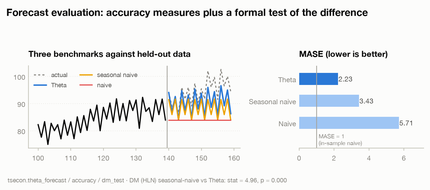
The gallery figure shows this exact exercise: Theta captures both the trend and the seasonal shape while the naive methods each miss one, and the MASE panel quantifies it (Theta 2.23 against the seasonal naive's 3.43 and the naive's 5.71, with a Diebold-Mariano statistic of 4.96, p < 0.001 — both tools defined next).
⚠ Common mistake. Publishing a forecast evaluation with no benchmark column. An RMSE in isolation is uninterpretable; the reader cannot tell whether your model added anything over "tomorrow equals today." The macro literature's convention — report RMSE ratios against a random walk (Atkeson and Ohanian 2001 made this famous for inflation) — exists precisely because bare loss numbers hide the benchmark comparison.
Scoring the errors: accuracy measures and their failure modes
You care about the choice of accuracy measure because measures disagree — a model can win on absolute error and lose on squared error, and cross-series comparisons are meaningless under the wrong measure. Given evaluation errors \(e_i = y_i - \hat{y}_i\), \(i = 1, \dots, P\):
RMSE punishes large errors disproportionately (it is the loss that the conditional mean forecast optimizes); MAE treats all errors linearly (the median forecast's loss). Both are scale-dependent: an RMSE of 0.4 is excellent for quarterly GDP growth and absurd for the level of the S&P 500, so neither can be averaged across series of different scales.
The traditional fix, MAPE (mean absolute percentage error), divides each error by the actual value — and fails exactly where practitioners need it. If any actual is zero the measure is undefined; if actuals are near zero it explodes; and it is asymmetric, penalizing over-forecasts more than under-forecasts of the same size because the actual, not the forecast, sits in the denominator (Goodwin and Lawton 1999; Hyndman and Koehler 2006). The "symmetric" sMAPE used in the M-competitions patches the zero problem but is not actually symmetric. tsecon computes both for compatibility and simply omits them from the result when a zero denominator would poison them.
Hyndman and Koehler (2006) proposed the clean solution, MASE (mean absolute scaled error): scale the out-of-sample errors by the in-sample MAE of the seasonal naive forecast,
where the denominator is computed on the training sample with seasonal period \(m\). MASE is scale-free (safe to average across series — it is the official metric of the recent M-competitions, with its squared-error sibling RMSSE the M5 metric) and self-benchmarking: MASE \(= 1\) means "exactly as accurate as a naive forecaster who saw only the training data," so anything above 1 is a red flag you can read without context.
for name, fc in [("Theta", fc_theta), ("seasonal naive", fc_snaive), ("naive", fc_naive)]:
    acc = tsecon.accuracy(test, fc, insample=train, period=4)
    print(f"{name:16s} RMSE {acc['rmse']:6.2f}   MAE {acc['mae']:6.2f}   MASE {acc['mase']:5.2f}")
accuracy returns me (mean error — bias, worth checking separately: a model can have a small RMSE and still be systematically too high), rmse, mae, mape/smape when defined, and mase/rmsse when a training sample is supplied.
For interval and density forecasts the scoring logic generalizes. The pinball loss (quantile loss) scores a forecast of the \(\tau\)-quantile:
which penalizes being on the wrong side of the realization asymmetrically — exactly the asymmetry that makes the \(\tau\)-quantile the optimal forecast under it. Averaging pinball loss over a fine grid of quantiles approximates (half of) the CRPS, the continuous ranked probability score, which scores an entire predictive distribution at once: it is the squared distance between the forecast CDF and the degenerate "step function at the realization," and it collapses to absolute error when the forecast is a point. CRPS is proper — no forecaster can improve their expected score by reporting a distribution other than their honest belief (Gneiting and Raftery 2007) — which is the non-negotiable requirement for any density score. Pinball loss and CRPS are roadmap items; the concepts are here because you should demand them from any density forecast you are shown.
⚠ Common mistake. Averaging MAPE over a panel that contains near-zero actuals (inflation around zero, growth rates in recessions): a handful of exploding terms dominates the average, and the model ranking becomes a ranking of who got lucky on the small-denominator months. Use MASE. Relatedly: never average raw RMSE across series of different scales — the largest-scale series simply wins.
Is the difference real? The Diebold-Mariano test
Your model's MASE is 2.23 and the benchmark's is 3.43. Over only 20 evaluation points, could that gap be luck? Accuracy tables without significance tests invite overreading — this is the forecasting analogue of reporting coefficients without standard errors.
Diebold and Mariano (1995) reduced the question to something elegant. Take two forecast error streams \(e_{1t}\) and \(e_{2t}\), pick a loss function \(L\) (squared or absolute), and form the loss differential
The null of equal predictive accuracy is simply \(E[d_t] = 0\) — a hypothesis about the mean of one observable series, no matter how complicated the models behind the forecasts are. The test statistic is a t-statistic on \(\bar{d}\),
where the denominator uses a long-run variance (Chapter 3's HAC machinery) because \(d_t\) is autocorrelated — mechanically so for \(h\)-step forecasts, whose errors overlap by MA(\(h-1\)) as we saw. Harvey, Leybourne and Newbold (1997) showed the raw statistic over-rejects in small samples and derived a correction: rescale by \(\sqrt{(P + 1 - 2h + h(h-1)/P)/P}\) and compare against Student-\(t\) with \(P-1\) degrees of freedom. tsecon applies HLN by default — it is not an option you can forget to enable:
dm = tsecon.dm_test(test - fc_snaive, test - fc_theta, h=1, loss="squared")
dm["hln_stat"], dm["p_value"]      # HLN-corrected statistic, t(P-1) two-sided p
dm["mean_loss_diff"]               # positive: the SECOND stream (Theta) had lower loss
The sign convention: \(d_t\) is loss of the first stream minus loss of the second, so a positive statistic favors the second argument. (This snippet, mirroring the gallery, pools all 20 horizons into one comparison for simplicity; a per-horizon evaluation from a proper backtest — one DM test per horizon, or the joint multi-horizon tests in the frontier — is the rigorous version.)
Two caveats keep DM honest. First, nested models: if model 2 is model 1 plus extra predictors, then under the null the extra coefficients are zero, the two forecasts converge to being identical, and \(d_t\) degenerates — the DM statistic has no proper distribution and is biased against the larger model, whose estimation noise inflates its MSE. Clark and West (2006, 2007) fixed this with an adjusted loss differential,
which adds back the estimation-noise term. Clark-West ships as tsecon.cw_test(e_small, e_large, yhat_small, yhat_large) — it needs the two forecasts as well as the two error streams, because the correction term is built from their difference — and the next section runs it. Never run plain DM on a nested comparison; run cw_test. Second, multiple comparisons: run DM against a benchmark for 50 candidate models and at the 5% level roughly two or three "significant" winners appear under the null by construction. The honest tools ship: spa_test (White's 2000 Reality Check and Hansen's 2005 test for Superior Predictive Ability, which ask whether the BEST of \(m\) models beats the benchmark once the search over all \(m\) is accounted for), stepm_test (Romano-Wolf 2005: which models beat it, at a controlled family-wise error rate) and model_confidence_set (Hansen, Lunde and Nason 2011, which reports the set of models statistically indistinguishable from the best) — see the section below. The discipline they formalize costs nothing even before you run them: count every specification you tried, not just the survivors, and treat a lone marginal DM rejection from a large search as noise. Diebold's own retrospective (Diebold 2015) is blunt that the test compares forecasts, not models — it takes the error streams as given, which is exactly why it is so widely applicable and so widely misapplied.
⚠ Common mistake. Running a plain DM test on nested models (an AR(2) against the same AR(2) plus an unemployment gap, say). The comparison feels natural — it is the most common question in applied work — but it is precisely the degenerate case. Nothing stops you:
dm_testtakes error streams and cannot know where they came from, so it will return a p-value that looks perfectly ordinary. Recognizing nestedness and reaching forcw_testis your job today; having the backtest object route the comparison automatically is the roadmap item.
The nested case, run three ways
Here is the degeneracy on the chapter's quarterly recipe, with the null true by construction. The small model is an AR(1); the large model is the same AR(1) plus one extra regressor that is pure noise. A fixed rolling window is used throughout, because the third test below requires it. This block rebuilds its own series, so it runs on its own:
import numpy as np, tsecon

g = np.random.default_rng(7)                       # the quarterly recipe from earlier
T = 160
ti = np.arange(T)
sn = 4.0 * np.array([1.0, -0.4, 0.6, -1.2])[ti % 4]
nz = np.zeros(T)
u = g.standard_normal(T)
for i in range(1, T):
    nz[i] = 0.6 * nz[i - 1] + 1.5 * u[i]
yq = 50 + 0.3 * ti + sn + nz

z = np.random.default_rng(99).standard_normal(T)   # an irrelevant predictor: the null is TRUE
W = 60                                             # fixed ROLLING width

tgt, f_small, f_large = [], [], []
for t in range(W, T - 1):
    sl = slice(t - W, t)                           # rolling window of width W
    Yw = yq[sl][1:]
    X_s = np.column_stack([np.ones(W - 1), yq[sl][:-1]])
    X_l = np.column_stack([X_s, z[sl][:-1]])
    b_s = tsecon.ols(Yw, X_s)["params"]
    b_l = tsecon.ols(Yw, X_l)["params"]
    tgt.append(yq[t])
    f_small.append(b_s[0] + b_s[1] * yq[t - 1])
    f_large.append(b_l[0] + b_l[1] * yq[t - 1] + b_l[2] * z[t - 1])
tgt, f_small, f_large = map(np.asarray, (tgt, f_small, f_large))
e_small, e_large = tgt - f_small, tgt - f_large

dmn = tsecon.dm_test(e_small, e_large, h=1, loss="squared")
cwn = tsecon.cw_test(e_small, e_large, f_small, f_large)     # needs the forecasts too
gwn = tsecon.gw_test(e_small ** 2, e_large ** 2)             # any two loss streams

print(f"origins {len(tgt)}")
print(f"MSE  small {np.mean(e_small**2):.3f}   large {np.mean(e_large**2):.3f}")
print(f"DM (HLN)  stat {dmn['hln_stat']:+.3f}   p {dmn['p_value']:.3f}")
print(f"CW        stat {cwn['cw_stat']:+.3f}   p {cwn['p_value']:.3f}")
print(f"GW        stat {gwn['gw_stat']:.3f}    p {gwn['p_value']:.3f}")
origins 99
MSE  small 50.617   large 53.100
DM (HLN)  stat -2.653   p 0.009
CW        stat -2.441   p 0.993
GW        stat 7.113    p 0.008
Read those three lines carefully, because they are three different questions, not three attempts at one.
DM is the one that misleads. The extra regressor is noise, so in population the two models are identical — yet the large model's MSE is about 2.5 higher (53.100 against 50.617), purely because it burns a degree of freedom estimating a coefficient that should be zero. DM takes that estimation noise at face value and reports the large model significantly worse (\(p = 0.009\)). That is the nested-model bias, visible: the statistic is not testing what it looks like it is testing.
cw_test is the fix, and it is one-sided. Its null is "the small model is as good," so a large positive statistic is evidence the extra predictor helps. Here \(-2.44\) with \(p = 0.993\) correctly refuses to reject — the adjustment adds back exactly the \((\hat{y}_1 - \hat{y}_2)^2\) term DM was charging to the large model. Do not read the near-1 p-value as "the small model won significantly"; a one-sided test that fails to reject is silent, not affirmative.
gw_test rejects, and is also right. Giacomini-White tests the forecasting method — estimation window and all — so its null is a statement about the procedure you would actually run, and under a fixed rolling window the cost of estimating a useless coefficient never washes out. "The large method forecasts worse" (\(\chi^2(1) = 7.11\), \(p = 0.008\)) and "the extra predictor has no population content" (CW) are both true. That is why the scheme matters: gw_test is only valid on the fixed-width rolling design used above, which is the frontier section's point made concrete.
Combining forecasts: the free lunch that mostly is
When several plausible models disagree, the instinct is to pick the best one. Half a century of evidence says: don't — average them. Bates and Granger (1969) made the point analytically: any convex combination of two unbiased forecasts has an error variance no worse than the better component whenever the forecasts are not perfectly correlated, because their idiosyncratic errors partially cancel. The optimal weights depend on the error covariance matrix — and here practice delivered one of the field's great running jokes, the forecast combination puzzle: estimated "optimal" weights routinely forecast worse than a plain equal-weighted average. The resolution is not mysterious — optimal weights must be estimated, weight-estimation error swamps the modest gains the true weights would deliver, and \(1/N\) has zero estimation error (Smith and Wallis 2009; Claeskens et al. 2016). Stock and Watson (2004), combining forecasts across seven countries' output growth, found simple averages hard to beat with anything clever.
fc_combo = 0.5 * fc_theta + 0.5 * fc_snaive          # the humble 1/N combination
for name, fc in [("Theta", fc_theta), ("seasonal naive", fc_snaive), ("combo", fc_combo)]:
    print(name, round(tsecon.accuracy(test, fc, insample=train, period=4)["mase"], 3))
(On this synthetic series Theta is so much better than the seasonal naive that averaging dilutes it — combination shines when components are comparably good and differently wrong. That, too, is a lesson: combination is insurance, not alchemy.)
The practical hierarchy, encoded in the roadmap's combination module: start with equal weights; consider the median or a trimmed mean if some forecasters occasionally produce wild outliers; estimate inverse-MSE (Bates-Granger) weights only with few forecasts and long track records; and treat regression-based weights (Granger and Ramanathan 1984) with suspicion unless constrained, because near-collinear forecasts make unconstrained weights explode.
⚠ Common mistake. Estimating combination weights on the same evaluation window you then report performance on. Weight estimation is model fitting; it must live inside the backtest's training windows like every other estimated quantity, or the combination's track record is contaminated by lookahead.
Are your densities honest? Calibration
A density forecast makes a quantitative promise at every probability level, and calibration checks whether the promises were kept: over many forecasts, realizations should fall below your reported 10th percentile 10 percent of the time, below the median half the time, and so on.
The universal diagnostic is the probability integral transform (PIT). For each forecast, evaluate your own predictive CDF at the realization:
If the density forecasts are correct, the \(u_t\) are independent uniform on \([0,1]\) at one-step horizons (Diebold, Gunther and Tay 1998). The histogram of PITs is then a lie detector with readable shapes: a hump in the middle means your densities are too wide (underconfident); a U-shape means too narrow (overconfident — realizations keep landing in your tails); a tilt means bias. Berkowitz (2001) sharpened this into a small-sample likelihood-ratio test by transforming PITs through the inverse normal CDF and testing for zero mean, unit variance, and no autocorrelation. One subtlety worth carrying even before the tools land: at horizons beyond one step, PITs are serially dependent under the null (overlapping errors again), so independence tests must be dropped and only uniformity tested.
Interval forecasts have their own proper score, worth knowing by name because it formalizes the intuition that a good interval is both narrow and reliable. The Winkler (1972) interval score for a central \((1-\alpha)\) interval \([l, u]\) charges the width plus a penalty of \(\frac{2}{\alpha}\) times the miss distance whenever the realization escapes:
A forecaster cannot game it: widening the interval buys fewer penalties but pays in width, and the exchange rate is calibrated so that reporting your honest quantiles is optimal.
Calibration alone is not enough — the unconditional historical distribution is perfectly calibrated and perfectly useless. The modern criterion is maximize sharpness subject to calibration (Gneiting's formulation): among honest densities, prefer the tightest. Proper scores like CRPS reward exactly this combination. PIT histograms, Berkowitz tests, and the scoring-rule battery are the density-evaluation core of Module 09.
Roadmap preview — this API lands with Module 09:
bt   = tsecon.backtest(y, window="expanding", train=80, horizon=8)   # ships today as a dict; Module 09 wraps it in a typed object
tab  = bt.accuracy()                      # per-horizon losses with HAC standard errors
test = bt.compare(benchmark, auto=True)   # auto-picks dm_test / cw_test / gw_test from the scheme; the tests themselves ship today
pits = bt.pit_histogram(bins=10)          # calibration diagnostics with binomial bands
⚠ Common mistake. Judging intervals by average coverage alone. A model can hit 95% coverage on average while its violations all cluster in recessions — precisely when the interval mattered. Conditional coverage (are violations independent over time?) is a separate, harsher question, and the clustered failures of Value-at-Risk models in 2008 are the canonical cautionary tale.
Backtesting in one call: the backtest engine
The hand-rolled POOS loop earlier in this chapter is the thing you should never have to write twice — get the slicing off by one and the whole track record is quietly wrong. The first slice of Module 09's engine has now landed as tsecon.backtest, and it turns that loop into a single call. It is deliberately function-shaped for now — an array in, a dict out — while the typed bt object with .compare() and .pit_histogram() shown in the roadmap preview above is still being built. What has landed is the part that is easy to get wrong by hand: the rolling-origin bookkeeping, the expanding/rolling schemes, the refit cadence, and the per-horizon accuracy table.
The signature mirrors the POOS design one-for-one:
tsecon.backtest(
    y,                       # the series (1-D)
    window="expanding",      # "expanding" (recursive) or "rolling" (fixed width)
    train=20,                # first training window (min_train if expanding, width if rolling)
    horizon=1,               # evaluate horizons 1..=horizon at every origin
    refit_every=1,           # re-estimate the forecaster every k origins (1 = every origin)
    forecaster=None,         # None ("naive") | drift | mean | seasonal_naive | theta | a callable
    period=None,             # seasonal period — "seasonal_naive"/"theta" ONLY; see below
    insample_period=1,       # seasonal period for the MASE/RMSSE scaling denominator
)
Those are the real defaults, and one of them bites: period belongs to the two seasonal forecasters alone. Pass it alongside forecaster="naive" (or a callable) and the call raises rather than silently ignoring it, because a silently-ignored seasonal period is the kind of argument slip that produces a wrong-looking benchmark table you cannot explain. The MASE/RMSSE scaling season is the separate insample_period, which is always live.
forecaster also accepts any Python callable — the hook for running a real model (statsmodels, scikit-learn, your own estimator) through this engine's leakage discipline. The contract is forecaster(train, horizon) -> horizon point forecasts, where train is a read-only float64 array holding only that origin's training window; the engine never hands it anything after the origin, so every transformation, scaling, and hyperparameter choice written inside the closure is structurally prevented from peeking:
def ar2(train, horizon):                       # a two-lag least-squares forecaster
    X = np.column_stack([np.ones(len(train) - 2), train[1:-1], train[:-2]])
    b = tsecon.ols(train[2:], X)["params"]
    hist, out = list(train), []
    for _ in range(horizon):
        out.append(b[0] + b[1] * hist[-1] + b[2] * hist[-2])
        hist.append(out[-1])
    return out

bt_ar2 = tsecon.backtest(y, window="expanding", train=80, horizon=4,
                         forecaster=ar2, insample_period=4)
bt_ar2["accuracy"][0]["mase"]                  # 1.21 — the table below puts theta at 0.85 here
The return dict carries origins (the origin indices \(t\) actually evaluated), n_origins, horizon, forecasts and targets (each a list of horizon arrays, one row per horizon \(h\), aligned so that targets[h-1][i] - forecasts[h-1][i] is the error at origin origins[i] for step \(h\)), and accuracy — one row per horizon with me, mse, rmse, mae, mdae, and mape/smape/mase/rmsse wherever a denominator makes them well-defined.
The engine evaluates a rectangular origins-by-horizons grid: it keeps only origins that have all horizon targets in sample (the first full training window through index \(n-1-\text{horizon}\)), so every horizon's error stream has the same length and the same origins. That is not tidiness for its own sake — it is precisely what lets the Diebold-Mariano machinery downstream consume equal-length, index-aligned streams.
A per-horizon accuracy table
Reusing the quarterly trend-plus-season-plus-AR series from the backtesting section above:
bt = tsecon.backtest(y, window="expanding", train=80, horizon=4,
                     forecaster="theta", period=4, insample_period=4)

print(f"origins {bt['origins'][0]}..{bt['origins'][-1]}  ({bt['n_origins']} of them)")
for row in bt["accuracy"]:
    print(f"{row['name']:5s}  RMSE {row['rmse']:5.2f}  MAE {row['mae']:5.2f}  MASE {row['mase']:5.2f}")
#   h=1   RMSE  2.01  MAE  1.62  MASE  0.85
#   h=2   RMSE  1.85  MAE  1.43  MASE  0.75
#   h=3   RMSE  2.39  MAE  1.93  MASE  1.01
#   h=4   RMSE  2.21  MAE  1.75  MASE  0.92
Read the table down the horizon column, not across the loss columns. Theta's one-step MASE of 0.85 says it beats the in-sample seasonal-naive scale by about 15 percent; the numbers stay near or below 1 out to a year, which is the honest signal that the method has captured the trend and the seasonal shape rather than memorizing them. A table that started below 1 and blew past it by \(h=4\) would be telling you the method forecasts the next quarter but not the next year — a distinction the single-number RMSE from a one-step loop hides entirely.
Expanding versus rolling: the scheme is a modeling choice
window picks the origin scheme, and train means different things under each: the minimum (first) training size when expanding, the fixed width when rolling.
exp = tsecon.backtest(y, window="expanding", train=80, horizon=4, forecaster="theta", period=4, insample_period=4)
rol = tsecon.backtest(y, window="rolling",   train=60, horizon=4, forecaster="theta", period=4, insample_period=4)
exp["n_origins"], rol["n_origins"]      # (77, 97) — rolling starts earlier here (width 60 < min_train 80)
Expanding uses every observation and lets estimation error die away as the sample grows — the right default when you believe the parameters are stable. Rolling deliberately forgets, holding the window at a fixed width so old regimes cannot contaminate the fit — the right choice when you suspect the world changes. The choice is not only about robustness: as the frontier section notes, the Giacomini and White (2006) test of forecasting-method accuracy requires a fixed-width rolling window, because its asymptotics depend on estimation error not vanishing. If a gw_test comparison is where you are headed, back-test rolling from the start — window="rolling" is not a robustness variant there, it is the test's precondition.
Refit cadence: refit_every
Refitting a model at every one of hundreds of origins is often the expensive part of a backtest. refit_every=k re-estimates the forecaster once every \(k\) origins and rolls that fit's direct multi-step path forward in between — the horizon-\(h\) forecast for the \(s\)-th origin after a refit is read off step \(s+h\) of the fit made at the refit origin.
fresh = tsecon.backtest(y, train=80, horizon=4, refit_every=1, forecaster="theta", period=4, insample_period=4)
stale = tsecon.backtest(y, train=80, horizon=4, refit_every=4, forecaster="theta", period=4, insample_period=4)
fresh["accuracy"][0]["rmse"], stale["accuracy"][0]["rmse"]   # (2.01, 2.17) — staleness costs a little accuracy
The default refit_every=1 is the leakage-free ideal: every origin sees a model fit on exactly its own training window. Larger \(k\) trades a little accuracy (the fit is up to \(k-1\) origins stale) for a large speed-up, and is how you make a full-competition backtest tractable; report the cadence you used, because it is part of the experiment.
The benchmark zoo, now callable
The five forecasters that populate the benchmark floor — naive, drift, mean, seasonal_naive, theta — are all reachable through the same call, so the mandatory "did I beat the dumb methods?" table is one loop:
print(f"{'forecaster':15s}  RMSE(h=1)  MASE(h=1)")
for fc in ["naive", "drift", "mean", "seasonal_naive", "theta"]:
    seasonal = {"period": 4} if fc in ("seasonal_naive", "theta") else {}   # period is theirs alone
    bt = tsecon.backtest(y, window="expanding", train=80, horizon=4,
                         forecaster=fc, insample_period=4, **seasonal)
    h1 = bt["accuracy"][0]
    print(f"{fc:15s}   {h1['rmse']:6.2f}    {h1['mase']:6.2f}")
# naive             6.74      3.36
# drift             6.76      3.37
# mean             18.57      9.42
# seasonal_naive    2.45      1.01
# theta             2.01      0.85
The ranking is a compressed lesson in why the benchmark you pick matters. On a trending, seasonal series the historical mean is a disaster (MASE 9.42 — it forecasts a flat line through data that is climbing), naive and drift are mediocre because they ignore the season, seasonal_naive is respectable (MASE ≈ 1, by construction near the scaling benchmark), and only theta clears the bar with room to spare. Swap in a random walk with no drift and the ranking inverts — which is the whole point of always reporting against a panel of benchmarks rather than a single favorite. Note the seasonal guard in the loop: period is only accepted by seasonal_naive and theta, so a loop that passes it to all five raises on the first iteration rather than quietly mis-scoring the non-seasonal three.
From the backtest straight into Diebold-Mariano
Because the grid is rectangular and index-aligned, wiring the backtest's error streams into the dm_test from earlier in the chapter is mechanical: run the benchmark and the challenger with the same scheme, subtract to get the per-horizon error streams, and hand them to dm_test with the matching h so the HLN correction uses the right MA(\(h-1\)) overlap.
H = 4
challenger = tsecon.backtest(y, train=80, horizon=H, forecaster="theta",          period=4, insample_period=4)
benchmark  = tsecon.backtest(y, train=80, horizon=H, forecaster="seasonal_naive", period=4, insample_period=4)
assert challenger["origins"] == benchmark["origins"]      # same scheme => same, aligned origins

print("h   DM(HLN)   p")
for h in range(1, H + 1):
    e_bench = np.array(benchmark["targets"][h - 1])  - np.array(benchmark["forecasts"][h - 1])
    e_chall = np.array(challenger["targets"][h - 1]) - np.array(challenger["forecasts"][h - 1])
    dm = tsecon.dm_test(e_bench, e_chall, h=h, loss="squared")   # positive stat favors the 2nd stream (theta)
    print(f"{h}   {dm['hln_stat']:6.3f}   {dm['p_value']:.4f}")
# h   DM(HLN)   p
# 1    2.111   0.0381
# 2    3.246   0.0017
# 3    0.407   0.6850
# 4    2.246   0.0276
This is the rigorous version of the pooled DM snippet from the Diebold-Mariano section: one test per horizon, each on a clean, equal-length error stream, rather than one comparison stapling all horizons together. Theta significantly beats the seasonal naive at \(h=1,2,4\) but not at \(h=3\) — the kind of horizon-specific verdict a single pooled statistic averages away. (Running \(H\) separate tests reopens the multiple-comparison problem the DM section flagged; Quaedvlieg's (2021) joint multi-horizon test, a roadmap item, is the honest way to control family-wise error across the horizon block.)
⚠ Common mistake. Comparing two backtests run under different schemes or training windows and then subtracting their error streams. Change
windowortrainand the surviving origins change, the twooriginslists no longer match, and the differenced series is nonsense even though the arithmetic runs. Assert equaloriginsbefore differencing — as above — every single time.
A few caveats to carry. backtest scores point accuracy only — the built-in forecasters are point forecasters, and a callable returns points — so density scoring (PITs, CRPS, the interval score) is still roadmap; distribution-free intervals around any of these forecasters are not, and are the next section. The MASE and RMSSE denominators are computed once, from the first training window at insample_period, never from the test sample — the correct, leakage-free convention, but it means the scaling reflects the earliest window's seasonality. The engine refuses degenerate designs loudly rather than returning a short or empty track record: ask for a horizon so long that no origin has all its targets in sample and it raises a ValueError that names the exact index arithmetic and tells you to lengthen the series, shrink the window, or shorten the horizon. And the leakage guarantee is structural for the callable hook too, precisely because the closure only ever receives its own training slice: every transformation, scaling, and hyperparameter choice must live inside it — the same discipline the manual-loop warning demanded, now the engine's contract (Tashman 2000). A callable that raises aborts the backtest and is re-raised naming the failing origin and window, so a bad model does not quietly produce a short track record.
Many models at once: SPA, StepM and the Model Confidence Set
Every table above compares two forecasters. Real work compares ten or fifty, and the moment you scan a column of DM p-values for the smallest one, the p-values stop meaning what they say: search over \(m\) candidates and the best of them beats the benchmark at 5% by luck alone with probability far above 5%. Three tests fix this, and all three take exactly the object the backtest loop already produces — a \(T \times m\) table of per-origin losses.
spa_test asks the joint question. With \(d_{t,k} = L_t(\text{benchmark}) -
L_t(\text{model }k)\) (positive favours the model), the null is
\(H_0: \max_k \mathbb{E}[d_k] \le 0\) — no model beats the benchmark — and the
statistic is the maximum of the standardized mean loss differentials. Its null
distribution comes from a block bootstrap of the whole loss panel with rows resampled
together, so the cross-model correlation that shapes a maximum is preserved. White's
(2000) Reality Check re-centres every model to zero; Hansen's (2005) SPA adds the
insight that models significantly worse than the benchmark should not be re-centred
at all, because padding the comparison with junk should not make a real winner harder
to detect. That gives the three p-values the call returns — p_value_upper (White,
conservative), p_value_consistent (Hansen, the recommended one, also returned as
p_value) and p_value_lower (the liberal bound) — which always satisfy
\(p_\text{lower} \le p_\text{consistent} \le p_\text{upper}\).
stepm_test answers the follow-up. A rejection says someone beat the benchmark;
Romano and Wolf's (2005) stepwise procedure says who, controlling the family-wise
error rate across the whole set of claims. That control is asymptotic, and tsecon
measures it rather than assuming it: with 200 observations, five models and
autocorrelated losses, the un-studentized rule (studentize=False) named at least
one model that was not really better in 6.25% of samples at size=0.05 when every
model tied the benchmark — arch's own StepM: 5.7% — while the studentized default
did so in 10.25%, falling to 6.5% at 800 observations (the forecasting model card has
the four-design table).
model_confidence_set drops the benchmark entirely. Given the same loss table it
returns the set of models that cannot be distinguished from the best at level size,
by repeatedly testing equal predictive ability across the survivors and eliminating
the worst when the test rejects. Each model gets an MCS p-value — the running
maximum of the step p-values along the elimination path — so one call describes every
size at once: the set at any \(\alpha\) is \(\{k : p_{\text{MCS}}(k) > \alpha\}\), and the
sets are nested in \(\alpha\). This is the honest answer to "which model should I use?"
when the data cannot single one out.
Wiring the benchmark zoo into all three is the same rectangular-grid trick the DM
section used — one backtest per forecaster under one scheme, then np.column_stack:
names = ["naive", "drift", "mean", "seasonal_naive", "theta"]
losses, origins = [], None
for fc in names:
    seasonal = {"period": 4} if fc in ("seasonal_naive", "theta") else {}
    bt = tsecon.backtest(y, window="expanding", train=80, horizon=1,
                         forecaster=fc, insample_period=4, **seasonal)
    assert origins is None or bt["origins"] == origins       # same scheme => aligned
    origins = bt["origins"]
    err = np.array(bt["targets"][0]) - np.array(bt["forecasts"][0])
    losses.append(err ** 2)                                  # squared-error loss column
L = np.column_stack(losses)                                  # the 80 x 5 loss table

mcs = tsecon.model_confidence_set(L, size=0.10, reps=2000, seed=0)
print(f"{'forecaster':16s} mean loss   MCS p   in the 90% set?")
for k, nm in enumerate(names):
    print(f"{nm:16s} {mcs['mean_losses'][k]:8.2f}   {mcs['mcs_p_values'][k]:5.3f}   "
          f"{'yes' if k in mcs['included'] else 'no'}")
print("eliminated, worst first:", [names[k] for k in mcs["elimination_order"]])
# forecaster       mean loss   MCS p   in the 90% set?
# naive               45.73   0.000   no
# drift               46.06   0.000   no
# mean               351.11   0.000   no
# seasonal_naive       5.93   0.024   no
# theta                4.03   1.000   yes
# eliminated, worst first: ['drift', 'naive', 'mean', 'seasonal_naive', 'theta']
The 90% model confidence set on this series is a single model. That is the strongest
verdict an MCS can deliver, and it is the same conclusion the benchmark table
reached — but now with the search accounted for, and with seasonal_naive excluded on
a p-value (0.024) rather than on eyeballing a 5.93-against-4.03 gap. Read the
elimination order as a diagnostic, not a ranking: drift goes first even though
mean has eight times its loss, because the range statistic eliminates the worst
member of the most standardized pair, and mean's enormous loss variance keeps its
standardized differences down. The ranking you want is mean_losses; the evidence
is in mcs_p_values.
Against a named benchmark the same table feeds spa_test and stepm_test:
spa = tsecon.spa_test(L[:, 3], L[:, [0, 1, 2, 4]], reps=2000, seed=0)   # vs seasonal_naive
print(spa["statistic"], spa["p_value"], spa["p_value_upper"], spa["best_model"])
# 2.151  0.019  0.046  3        (best_model 3 = theta, the 4th column passed)
tsecon.stepm_test(L[:, 3], L[:, [0, 1, 2, 4]], size=0.05, reps=2000, seed=0)["superior_models"]
# [3]                           theta, and only theta, beats the seasonal naive at FWER 5%
Note the gap between the consistent p-value (0.019) and White's (0.046): three of the four candidates are far worse than the benchmark, and re-centring them — as the Reality Check does — inflates the simulated maximum and costs power. That gap is Hansen's whole point, and it grows with the number of junk models in your search.
Three practical warnings. First, block_size=None picks the Politis-White optimal
length per column and averages; it is a good default but the bootstrap's block length
is the one setting that moves these p-values, so report it (it comes back in
block_size) and check that a hand-set length near \(n^{1/3}\) tells the same story.
Second, the tests take the loss table as given — they cannot know the forecasts came
from nested models, so the cw_test warning from earlier still applies to each
column. Third, studentize=True (the default, Hansen's own statistic) divides both
the observed statistic and every bootstrap replicate by the same estimated long-run
standard deviation, which over-rejects in small samples; the model card measures how
much, and studentize=False gives White's un-studentized statistic, which is what
arch computes and what our goldens pin exactly.
Distribution-free intervals: conformal prediction
Everything above scored points. The moment you want an interval, you owe the reader a distributional assumption — Gaussian errors, a fitted density, a bootstrap — and on economic data those assumptions are exactly what fails in the tail. Conformal prediction buys an interval without one: run your forecaster over a calibration stretch, collect its realized \(h\)-step residuals, and band the forward forecast with an order statistic of those residuals. Under exchangeability the coverage guarantee is finite-sample and assumption-free (Vovk et al. 2005). Time series are not exchangeable, so the guarantee is approximate rather than exact here — which is a reason to measure the coverage, not a reason to skip the method.
conformal_forecast ships all three of the standard variants, wrapped around any of the backtest forecasters (or your own callable):
split = tsecon.conformal_forecast(y, horizon=4, alpha=0.1, base="theta", period=4, calib=40)
print(np.round(split["lower"], 2), np.round(split["upper"], 2))
# [99.8  92.46 97.7  88.42] [106.88  98.91 105.61  95.5 ]
print(split["level"], round(split["finite_sample_level"], 4), split["n_calib"])
# 0.9 0.9024 40   <- the (m+1)(1-alpha)/m order statistic, not the plain 90th percentile

aci = tsecon.conformal_forecast(y, horizon=1, alpha=0.1, base="theta", period=4,
                                method="aci", calib=40, n_eval=40)
enb = tsecon.conformal_forecast(y, horizon=1, alpha=0.1, method="enbpi",
                                base="ar", lags=4, n_boot=30, seed=0)
print(np.round(aci["alpha_final"], 3), np.round(enb["lower"], 2), np.round(enb["upper"], 2))
# [0.1] [96.4] [102.83]
method="split"is the baseline: hold out the lastcaliborigins under the backtest engine's own leakage discipline, then band the forward forecast with the finite-sample-corrected quantile of the absolute residuals — the \(\lceil (m+1)(1-\alpha) \rceil\)-th smallest, which is whyfinite_sample_levelreads 0.9024 rather than 0.90 at \(m = 40\). (mode="asymmetric"calibrates the two tails separately, and may then exclude a biased base's point forecast — that is the point.)method="aci"is adaptive conformal inference (Gibbs and Candès 2021): the working miscoverage level is nudged after every hit or miss, \(\alpha_{t+1} = \alpha_t + \gamma(\alpha - \mathrm{err}_t)\), so long-run coverage survives distribution shift. Here it wandered between 0.093 and 0.104 over the 40 evaluation origins (alpha_trajectory) and landed back at 0.10: this series is stable, so the adaptation had nothing to repair. On a series with drift it is the whole point.method="enbpi"(Xu and Xie 2021) builds the interval from a bootstrap ensemble's out-of-bag residuals with no sample splitting at all, and is seeded and bit-reproducible.
The honest companion is conformal_backtest, which forms the interval at each of the last n_eval origins from information available then and reports what coverage the method actually delivered:
cb = tsecon.conformal_backtest(y, horizon=1, alpha=0.1, base="theta", period=4,
                               calib=40, n_eval=40)
print(cb["realized_coverage"], int(np.sum(cb["err"][0])))
# [0.9] 4     <- 36 of 40 intervals covered, against a promised 0.90
That is the number to publish. A conformal interval is only as good as its realized coverage on your series, and the gap between the nominal level and the measured one is the honest measure of how far from exchangeable your data is.
⚠ Common mistake. Reading the split-conformal guarantee as if it held on time series. It is a theorem about exchangeable scores; forecast residuals from a persistent, drifting series are not exchangeable, and the coverage you get is empirical, not guaranteed. Run
conformal_backtestbefore you quote a level — and if realized coverage sags, reach formethod="aci", which is built for exactly that failure.
Forecasting an event, not a level: recession probabilities
Every forecast so far in this chapter has aimed at a number — a level, a growth rate, a point on a continuous scale, scored by how far it lands from the realization. But some of the most consequential forecasts in macroeconomics are about a binary event: will the economy be in recession next quarter? The target is 0 or 1, and squared error against a 0/1 outcome is the wrong instrument. What you want is a probability, and a probability is judged by calibration — did the quarters you called 30 percent recession risk turn out to be recessions about 30 percent of the time? — not by its distance from the realized 0 or 1.
The workhorse for this is the binary-choice model, and the leading indicator is one you already know from the yield-curve chapter: the term spread, the long yield minus the short yield. An inverted curve — a negative spread, short rates above long — has preceded almost every postwar US recession, and a single-regressor term-spread probit (Estrella and Mishkin 1998) is still a staple of central-bank recession dashboards. The model runs a linear index of leading variables through a probit or logit link and reads off a recession probability:
with \(\Phi\) the standard normal CDF (a logit swaps in the logistic CDF; the coefficients land on a different scale — roughly \(1.6\times\) the probit's — but the fitted probabilities are close). A negative coefficient on the spread is the whole story: the lower the spread, the higher the index, the higher \(\Phi(\cdot)\), the higher the recession probability.
recession_probit fits this by maximum likelihood. The object you actually use is probabilities — the fitted \(P(y_t=1)\) path you plot or threshold — and the coefficients come with zstats for the usual asymptotic z-tests. Fit quality is reported as McFadden's pseudo-\(R^2\), \(1 - \ell/\ell_0\) (the fitted log-likelihood over the intercept-only one). It is not the ordinary \(R^2\) and does not live on the same scale: values of 0.2–0.4 are strong for binary choice, so do not be alarmed that a genuinely useful recession model scores what would be a mediocre \(R^2\) in a level regression.
import numpy as np
import tsecon

rng = np.random.default_rng(11)
n = 400
spread = np.zeros(n)                              # term spread: a persistent leading indicator
for t in range(1, n):
    spread[t] = 0.7 * spread[t - 1] + rng.standard_normal()

index = -0.8 - 1.0 * spread                       # inverted curve (low spread) -> higher recession risk
y = (index + rng.standard_normal(n) > 0).astype(float)
print(f"recession share in sample: {y.mean():.2f}")

X = np.column_stack([np.ones(n), spread])         # STATIC probit: X MUST carry the constant column
fit = tsecon.recession_probit(y, X, link="probit")
print("params [const, spread]:", np.round(fit["params"], 3))
print("z-stats               :", np.round(fit["zstats"], 3))
print(f"pseudo-R2 = {fit['pseudo_r2']:.3f}")
print("first 3 fitted P(recession):", np.round(fit["probabilities"][:3], 3))
# recession share in sample: 0.27
# params [const, spread]: [-0.9   -1.056]
# z-stats               : [-9.177 -9.899]
# pseudo-R2 = 0.393
# first 3 fitted P(recession): [0.184 0.175 0.009]
The spread coefficient is \(-1.06\) with a z-statistic near \(-10\): strongly negative, exactly the inverted-curve signal. The pseudo-\(R^2\) of 0.39 is excellent for a recession probit, and probabilities is the calibrated risk series a policymaker reads month by month.
Static or dynamic: does recession pressure persist on its own?
The static model treats each quarter's recession risk as a function of today's indicators alone. But recessions are sticky in a way the leading indicators do not fully capture: being in a downturn this quarter makes one next quarter more likely, over and above whatever the spread is saying. The Kauppi-Saikkonen (2008) dynamic probit builds that persistence into the index itself, giving it an autoregressive term:
Here \(\rho\) measures how much recession pressure carries over period to period. It nests the static probit at \(\rho = 0\), so on persistent data it can only fit better — and flipping dynamic=True switches to it. The one rule that bites: the static model needs a constant column in x, and the dynamic model must not have one, because it estimates its own intercept \(w\) and a redundant constant makes the information matrix singular.
rng = np.random.default_rng(3)
n = 800
w, b, rho = -0.4, 1.1, 0.6
x = np.zeros(n)
for t in range(1, n):
    x[t] = 0.6 * x[t - 1] + rng.standard_normal()
y = np.zeros(n)
prev = w / (1 - rho)                              # stationary-mean initialization
for t in range(n):
    idx = w + b * x[t] + rho * prev               # the index carries its own lag
    y[t] = 1.0 if idx + rng.standard_normal() > 0 else 0.0
    prev = idx

Xd = x.reshape(-1, 1)                             # DYNAMIC probit: NO constant column
dyn = tsecon.recession_probit(y, Xd, dynamic=True)
print("params [w, b, rho]:", np.round(dyn["params"], 3))
print(f"rho = {dyn['rho']:.3f}   pseudo-R2 = {dyn['pseudo_r2']:.3f}")

stat = tsecon.recession_probit(y, np.column_stack([np.ones(n), x]))   # static comparison
print(f"loglik  dynamic {dyn['loglik']:.1f}  >=  static {stat['loglik']:.1f}")
# params [w, b, rho]: [-0.396  1.116  0.606]
# rho = 0.606   pseudo-R2 = 0.625
# loglik  dynamic -200.9  >=  static -323.3
The estimator recovers \(\rho \approx 0.61\) against the true 0.6, and the dynamic log-likelihood (\(-200.9\)) crushes the static one (\(-323.3\)) because the static model has no way to represent the recession's self-perpetuation. Reach for dynamic=True when downturns persist beyond what your covariates explain; if the data has no index persistence, \(\rho\) simply estimates near zero and you have lost nothing. Do not use either variant for a continuous target — this is classification, and a level forecast belongs to theta_forecast, var_forecast, and the rest of this chapter. The full argument contract, the separation failure mode, and the converged caveat live in the recession-probability model card.
⚠ Common mistake. Getting the constant column backwards. The static probit needs
xto include a column of ones; the dynamic probit must omit it. Include a constant in the dynamic model and the information matrix is singular; forget it in the static model and every coefficient is biased. It is the single most common way to misuserecession_probit.
Growth-at-risk: forecasting the downside
The recession probit collapses the future into a binary event. The workflow that has taken over policy institutions since 2019 keeps the whole distribution and asks a sharper question: how bad could growth plausibly get, given what financial conditions look like today? Adrian, Boyarchenko, and Giannone (2019) — "Vulnerable Growth," the paper behind the IMF's growth-at-risk surveillance and half the financial-stability reports now published — ran quantile regressions of future US GDP growth on the National Financial Conditions Index and found a striking asymmetry: tightening financial conditions drag down the lower quantiles of future growth far more than the median, while the upper quantiles barely move. The center of the forecast distribution is stable; its left tail breathes with financial stress. A mean forecast — even a perfect one — is structurally incapable of showing this.
The machinery is the quantile regression of Chapter 3, pointed at the future: for each \(\tau\) in a ladder, regress \(h\)-ahead growth on a constant, the conditions variables, and current growth,
and read the fitted quantiles, at every \(t\), as a conditional forecast distribution — a fan chart whose shape is allowed to depend on the state of the financial system. growth_at_risk runs the whole workflow in one call. On a synthetic quarterly economy built with the ABG asymmetry (tight conditions add a purely negative fat tail to future growth):
rng = np.random.default_rng(5)
T = 320                                        # 80 years of quarters
f = np.zeros(T)                                # financial-conditions index (high = tight)
y = np.zeros(T)                                # GDP growth, annualized
y[0] = 2.0
for t in range(1, T):
    f[t] = 0.8 * f[t - 1] + 0.6 * rng.standard_normal()
    downside = 0.9 * max(f[t - 1], 0.0) * abs(rng.standard_normal())   # stress fattens the LEFT tail only
    y[t] = 2.0 + 0.3 * y[t - 1] - 0.2 * f[t - 1] + rng.standard_normal() - downside

gar = tsecon.growth_at_risk(y, f.reshape(-1, 1), horizon=4)   # conditions is T x k
for i, tau in enumerate(gar["taus"]):                          # default taus: 5/25/50/75/95
    print(f"tau={tau}: conditions coeff {gar['params'][i][1]:+.3f}  (se {gar['bse'][i][1]:.3f})")

# tau=0.05: conditions coeff -0.829  (se 0.258)
# tau=0.25: conditions coeff -0.417  (se 0.133)
# tau=0.5: conditions coeff -0.324  (se 0.103)
# tau=0.75: conditions coeff -0.311  (se 0.134)
# tau=0.95: conditions coeff -0.362  (se 0.103)
The coefficient ladder is the ABG finding: a one-point tightening of conditions lowers median four-quarter growth by about 0.3, but lowers the 5th percentile by 0.83 — two and a half times as much, and about two standard errors of the 5th-percentile coefficient away from the median's. Financial stress is not a forecast of lower growth so much as a forecast of fatter downside risk.
Reading the output like a policy economist:
fit = np.array(gar["fitted"])                    # (n_taus, T): the fan at every observation
t_tight, t_calm = int(np.argmax(f)), int(np.argmin(f))
print(np.round(fit[:, t_tight], 2))              # [-3.51 -0.03  1.07  2.11  2.81]  f = +3.62
print(np.round(fit[:, t_calm], 2))               # [ 2.32  2.7   3.3   4.15  5.44]  f = -2.69

print(np.round(np.array(gar["current"]), 2))     # [0.09 1.48 2.42 3.25 4.52] — the latest risk read
print(gar["crossing"])                           # False — the raw quantile paths never crossed here
The two fans are the story in two lines. In the calmest quarter of the sample the 5-to-95 fan spans 2.3 to 5.4 — narrow, healthy, roughly symmetric around 3.3. In the most stressed quarter it spans \(-3.5\) to \(2.8\): the median has slipped about two points, but the 5th percentile has collapsed by nearly six — the fan does not shift, it smears leftward. And current is the number that goes in the briefing: conditional on the latest observation, the central expectation for growth a year out is 2.4, but there is a 5% risk it comes in at 0.1 or below. That 5th percentile is "growth-at-risk," the GaR(5%) that policy institutions now track the way they track the modal forecast.
Two mechanical notes. Because each \(\tau\) is fit separately, fitted quantile paths can cross; growth_at_risk applies the Chernozhukov–Fernández-Val–Galichon monotone rearrangement (a per-observation sort across \(\tau\)) by default, reports whether the raw paths crossed in crossing, and keeps the unsorted paths in fitted_raw so you can see what the rearrangement did — here it did nothing, because nothing crossed. And the fitted quantiles are forecasts, so they are scored like forecasts: with the pinball loss from the accuracy section at each \(\tau\), never with RMSE against the realization. Contract, validation, and the full ABG framing: the quantile model card. For the dynamic version of this question — how the whole quantile ladder responds horizon by horizon to an identified shock — see quantile local projections (quantile_lp) in Chapter 9.
⚠ Common mistake. Reading GaR(5%) as "the forecast." The 5th percentile is not what you expect to happen — it is the threshold below which outcomes should land one time in twenty, and if realized growth never comes in near your GaR estimates, your tail is too wide, not prudent. Calibration cuts both ways: over many quarters, roughly 5% of realizations should fall below the reported 5th percentile, and checking that (the pinball loss, the PIT machinery above) is what separates a risk measure from a scary number. Relatedly:
tausmust be strictly increasing, and extreme taus need long samples — the function refuses a 5th percentile the Hall-Sheather bandwidth cannot support rather than reporting one it cannot defend.
Are the forecasts themselves rational? Survey expectations
The whole chapter so far has compared models — is your VAR beating the random walk, is Theta beating the seasonal naive? A different and older question asks whether a set of published forecasts is rational on its own terms, without any competing model in sight. Given the Survey of Professional Forecasters, the Michigan survey, or a central bank's own projections, are those forecasts using information efficiently, or are they leaving predictable money on the table? Diebold-Mariano compares forecasts against each other; this family interrogates a single forecast against the standard of rationality.
The benchmark is full-information rational expectations (FIRE): a rational forecaster's error should be unpredictable from anything known when the forecast was made — including the forecaster's own past behavior. Two classic tests operationalize that, and both are OLS with a Newey-West (HAC) covariance, because forecast errors at overlapping horizons are serially correlated by construction (the same MA(\(h-1\)) overlap that has haunted every multi-step regression in this chapter).
Coibion-Gorodnichenko: do forecasters underreact?
The sharpest modern test regresses the mean forecast error on the mean forecast revision (Coibion and Gorodnichenko 2015):
Under FIRE the revision the consensus just made carries no information about the error it is about to realize, so \(\beta = 0\). A positive slope is the signature of information rigidity: forecasters underreact to news, so the direction they just revised predicts the error they are about to make. It is a beautiful test because the null does not care how the forecasts were made — it is a statement about the mean of one observable series. The estimator also reports the implied rigidity \(\beta/(1+\beta)\), which under sticky-information reads as the fraction of forecasters who did not update this period, and under noisy-information as the Kalman-gain complement — the same number, two stories.
One construction detail carries the identification: the revision in the paper is fixed-event — this vintage's forecast of a target minus last vintage's forecast of the same target, \(F_t x_{t+h} - F_{t-1} x_{t+h}\), which takes two horizons per survey round to build (the \(h\)-step forecast made at \(t\) and the \((h+1)\)-step forecast made at \(t-1\)). Differencing a single fixed-horizon series, \(F_t x_{t+h} - F_{t-1} x_{t+h-1}\), compares forecasts of different dates and is only an approximation whose slope is not the CG \(\beta\) in general — the expectations model card quantifies the bias on an exact sticky-information process.
rng = np.random.default_rng(0)
n = 200
rev = np.zeros(n); u = np.zeros(n)                # consensus revision (persistent) and a persistent error
for t in range(1, n):
    rev[t] = 0.5 * rev[t - 1] + rng.normal(0.0, 1.0)
    u[t]   = 0.6 * u[t - 1] + rng.normal(0.0, 0.8)
err = 0.1 + 0.7 * rev + u                          # true CG slope 0.7: forecasters underreact

cg = tsecon.cg_regression(err, rev)                # maxlags=None -> Newey-West rule-of-thumb bandwidth
print(f"CG slope {cg['slope']:.3f}  (HAC se {cg['se_slope']:.3f}, p {cg['p_slope']:.4f}), maxlags {cg['maxlags']}")
print(f"implied information rigidity = {cg['implied_rigidity']:.3f}")
# CG slope 0.699  (HAC se 0.085, p 0.0000), maxlags 4
# implied information rigidity = 0.411
The slope of 0.70 is precisely estimated away from zero: FIRE is rejected toward underreaction, and the implied rigidity of 0.41 says something like 40 percent of the information is stale each period. One caveat the model card stresses: this is a consensus-level test. Run the same regression on individual forecasters and the sign often flips to overreaction — a genuinely different exercise, not a bug.
Mincer-Zarnowitz: is the forecast even unbiased?
The older test asks the more basic question of efficiency: regress the forecast error on a constant and the forecast itself (or any information known at forecast time), and jointly test that all coefficients are zero. A rational forecast leaves errors that are mean-zero and unpredictable from the forecast, so a rejection says the forecast is systematically biased or inefficient with respect to those regressors.
rng = np.random.default_rng(1)
n = 200
fc = np.cumsum(rng.normal(0.0, 1.0, n)) * 0.3      # the forecasts
e = np.zeros(n)
for t in range(1, n):
    e[t] = 0.4 * e[t - 1] + rng.normal(0.0, 1.0)    # near-rational error
err = 0.15 + 0.05 * fc + e

mz = tsecon.forecast_efficiency(err, fc[:, None])   # regressors is T x k; the constant is added internally
print(f"Wald = {mz['wald']:.2f} on {mz['wald_df']} df, p = {mz['wald_pvalue']:.3f}")
print("coeffs [const, forecast]:", np.round(mz["params"], 3))
# Wald = 2.53 on 2 df, p = 0.282
# coeffs [const, forecast]: [-0.178 -0.039]
The Wald p-value of 0.28 does not reject: consistent with an efficient forecast, as designed. A rejection would tell you that the forecast is inefficient with respect to these regressors, not why — and the classic MZ regresses the outcome on the forecast to test intercept-and-slope \(=(0,1)\); the error-on-forecast form here is the algebraically equivalent restriction with a cleaner "all zero" null.
Disagreement: how far apart are the forecasters?
Rationality tests work on the consensus; a complementary and purely descriptive object is the cross-sectional disagreement — how much the individual forecasters spread out in each period. In sticky- and noisy-information models disagreement moves with the degree of information rigidity, so it is the natural companion series to the CG regression, and it doubles as an uncertainty proxy in downstream work. forecast_disagreement takes a ragged panel (one array of individual forecasts per period) and returns the within-period standard deviation and quartiles:
rng = np.random.default_rng(2)
panel = [rng.normal(2.0, s, 40) for s in (0.4, 0.8, 1.5)]   # three periods, each more dispersed
dis = tsecon.forecast_disagreement(panel)
print("std:", np.round(dis["std"], 3))
print("IQR:", np.round(dis["iqr"], 3), " counts:", list(dis["counts"]))
# std: [0.38  0.862 1.437]
# IQR: [0.506 1.38  2.09 ]  counts: [40, 40, 40]
Rising std or iqr is widening disagreement; prefer the IQR when a few extreme forecasters would otherwise dominate the standard deviation. Note the distinction the model card insists on: this is dispersion across forecasters, not the uncertainty of any single forecaster (which needs a density forecast) — do not conflate the two. Full argument contracts and validation for all three tools are in the survey-expectations model card.
⚠ Common mistake. Reading
implied_rigidityoff a negative CG slope. The formula \(\beta/(1+\beta)\) still returns a number, but the sticky/noisy-information interpretation only applies when the slope is positive (underreaction). A negative consensus slope — or the overreaction you tend to find on individual data — is a different phenomenon, not a rigidity to be reported.
The frontier
Three threads define the research edge of forecast evaluation.
The scheme decides the test. The DM test treats forecasts as primitives, but most forecasts come from estimated models, and estimation error contaminates the loss differential. West (1996) worked out the asymptotics when the null concerns population-level predictive ability: the correction depends on the ratio of evaluation to training sample sizes and on the origin scheme (recursive schemes let estimation error die away; fixed rolling windows keep it alive forever). Giacomini and White (2006) flipped the question — test the forecasting method, estimation window and all, in which case fixed-width rolling windows are not a nuisance but a requirement. Almost no software anywhere enforces the scheme-test match, which means published DM tests on nested, recursively estimated models — statistics whose asymptotics simply do not apply — are routine. Making the backtest object carry its scheme, and having tests refuse invalid combinations, is a central design commitment of Module 09.
Conformal prediction. A distribution-free answer to interval forecasting: compute your model's recent absolute residuals on a calibration window, take their 95th percentile \(q\), and report \(\hat{y} \pm q\). Under exchangeability this has a finite-sample coverage guarantee with no distributional assumptions (Vovk et al. 2005) — but time series are not exchangeable, so the guarantee formally fails exactly where economists need it. The repairs are online: adaptive conformal inference (Gibbs and Candès 2021) nudges the working miscoverage level after every hit or miss, restoring long-run coverage under arbitrary distribution shift; EnbPI (Xu and Xie 2021) builds intervals from bootstrap-ensemble residuals without sample splitting; conformalized quantile regression (Romano, Patterson and Candès 2019) handles heteroskedastic series. Split, ACI and EnbPI all ship — conformal_forecast and conformal_backtest, run in the conformal section above — and are the library's model-agnostic uncertainty layer. CQR is the piece still outstanding, along with conformal coverage bounds that degrade gracefully with the drift rather than merely being measured after the fact.
Honesty at scale and through time. Quaedvlieg (2021) replaced \(H\) separate per-horizon DM tests with joint multi-horizon comparisons controlling family-wise error across horizons. Giacomini and Rossi (2010) asked when rather than whether one model wins — a rolling DM statistic against sup-type bands that detects the breakdowns that full-sample averages wash out (predictability in macro is episodic; averaging over the Great Moderation and 2008 tells you little about either). Croushore and Stark (2001) showed model rankings can flip depending on which vintage of the data you evaluate against — GDP is revised for years, and a model evaluated against today's data saw numbers no real-time forecaster had. And anytime-valid e-value tests (Henzi and Ziegel 2022) let a dashboard ask "is the new model better yet?" every week without the repeated-testing penalty of classical p-values. All are roadmap items; none has a maintained open-source home today, which is much of the reason this module exists.
The honest open problems: evaluation under structural instability is unsolved in any general way (every full-sample average is a bet that the future resembles the average past); multiple-comparison corrections require knowing the true universe of specifications tried, which no tool can observe (the roadmap's evaluation registry is an attempt at infrastructure, not a solution); and conformal guarantees for genuinely nonstationary series remain partial — coverage bounds degrade with the drift, and quantifying the degradation is current research.
Which method when
| Situation | Reach for | Because |
|---|---|---|
| First forecast of a new series | theta_forecast + naive benchmarks |
The M3 winner and the mandatory floor; anything fancier must beat both |
| Comparing accuracy across series of different scales | MASE / RMSSE via accuracy(..., insample=train) |
Scale-free, self-benchmarking (1.0 = in-sample naive); MAPE explodes near zero |
| Deciding if a two-model accuracy gap is real (non-nested) | dm_test (HLN correction is the default) |
A t-test on the loss differential; HAC handles the overlap autocorrelation |
| Nested models (baseline vs baseline + extras) | cw_test(e_small, e_large, yhat_small, yhat_large) |
Plain DM is degenerate under the null; CW adds back the estimation-noise term. One-sided |
| Comparing forecasting methods, estimation error included | gw_test(loss1, loss2) on a fixed rolling-window backtest |
GW's null is about the procedure, so nestedness is not a problem — but the rolling scheme is a requirement |
| Many candidate models against one benchmark | spa_test / stepm_test; model_confidence_set for the set |
Pairwise DM tests ignore the search; SPA tests the maximum, StepM names the winners, MCS reports the statistically-best set |
| Multi-step forecast evaluation regressions | ols(..., se_type="hac", maxlags=h-1) |
Direct h-step errors are MA(h−1) by construction |
| Forecasting a small system of related variables | var_forecast |
Iterated multi-step point + interval forecasts from joint dynamics |
| Forecasting a binary business-cycle event (recession) | recession_probit |
Turns leading indicators (the term spread) into a calibrated P(recession); dynamic=True for persistence |
| Downside risk to growth from financial conditions | growth_at_risk |
ABG: conditions move the lower quantiles far more than the median; current is the latest conditional fan, and its 5th percentile is GaR(5%) |
| Testing whether published forecasts are rational | cg_regression, forecast_efficiency |
CG slope \(=0\) under FIRE (positive \(=\) underreaction); Mincer-Zarnowitz tests unbiasedness |
| Measuring dispersion across a forecaster panel | forecast_disagreement |
Cross-sectional spread — the empirical proxy for belief dispersion and information rigidity |
| Several plausible models, none dominant | Equal-weight average | The combination puzzle: 1/N beats estimated weights out of sample |
| Judging interval or density forecasts | conformal_backtest for realized coverage now; PITs, CRPS, Berkowitz (roadmap) |
Point measures cannot see whether the promised probabilities were kept |
| Valid intervals without a trusted distributional model | conformal_forecast (method="split", "aci", or "enbpi") |
Distribution-free calibration-window quantiles; ACI adapts the level under drift |
| Running a real model (statsmodels, sklearn) through an honest backtest | backtest(forecaster=<callable>) |
The callable only ever sees its own training slice, so preprocessing cannot leak |
| Suspecting the winner changed over time | Giacomini-Rossi fluctuation test (roadmap) | Full-sample averages hide episodic breakdowns in relative performance |
What tsecon implements today
Available now in Python (import tsecon):
theta_forecast(y, steps, period=1)— the Theta method, seasonal adjustment included; matches statsmodels'ThetaModel.accuracy(actual, forecast, insample=None, period=1)— ME, RMSE, MAE, MAPE and sMAPE (omitted on zero denominators rather than returning garbage), and MASE/RMSSE when a training sample is supplied.dm_test(e1, e2, h=1, loss="squared")— Diebold-Mariano with the HLN small-sample correction and \(t(P-1)\) p-values as the default, not an option;lossis"squared"or"absolute".cw_test(e_small, e_large, yhat_small, yhat_large, lrv_lags=0)— Clark-West for nested models: the adjusted differential \(e_1^2 - e_2^2 + (\hat{y}_1 - \hat{y}_2)^2\), returned ascw_stat/p_value(one-sided, null "the small model is as good") /mean_adj_diff. This is why it wants the forecasts and not only the errors. See the forecasting model card.gw_test(loss1, loss2, lrv_lags=0)— the Giacomini-White unconditional test of equal predictive ability on any two loss streams:gw_statis \(\chi^2(\text{df})\) withdf= 1. Valid for nested models provided the backtest used a fixed-width rolling window, because its null is about the forecasting method rather than the population model. The conditional GW test is still a roadmap item.var_forecast(data, lags=2, steps=8, alpha=0.05, trend="c")— iterated multi-step VAR forecasts with interval bands.recession_probit(y, x, link="probit", dynamic=False)— static probit/logit and the Kauppi-Saikkonen dynamic probit for a 0/1 recession indicator; returns the fittedprobabilities, coefficientzstats, and McFaddenpseudo_r2. See the recession model card.growth_at_risk(y, conditions, horizon=1, taus=..., rearrange=True)— the ABG conditional-quantile workflow: per-tauparams/bse, the fitted quantile fan at every observation (fitted, CFG-rearranged;fitted_rawunsorted;crossingflag), andcurrent, the risk read at the latest observation.conditionsis T x k. See the quantile model card.cg_regression(error, revision)andforecast_efficiency(error, regressors)— the Coibion-Gorodnichenko information-rigidity and Mincer-Zarnowitz rationality regressions (OLS with a Newey-West HAC covariance for the overlapping errors), plusforecast_disagreement(panel)for cross-forecaster dispersion. See the expectations model card.backtest(y, window=..., train=..., horizon=..., refit_every=..., forecaster=..., period=..., insample_period=...)— the rolling/expanding POOS engine: origin bookkeeping, refit cadence, a rectangular origins-by-horizons grid, and a per-horizon accuracy table.forecasteris one ofnaive/drift/mean/seasonal_naive/thetaor any Python callablef(train, horizon)that sees only its own training window.conformal_forecast(y, horizon=..., method="split"|"aci"|"enbpi", base=..., alpha=0.1, calib=..., mode=...)— distribution-free intervals around any of those forecasters (or a callablebase): split conformal with the finite-sample-corrected quantile, Gibbs-Candès adaptive conformal inference, and the seeded Xu-Xie EnbPI ensemble.conformal_backtest(...)— the same three methods run online over the lastn_evalorigins, returningrealized_coverageand the per-origin miss indicators: the honest grade for an interval method on your series.- Supporting cast from earlier chapters:
ols(..., se_type="hac", maxlags=...)for evaluation regressions with overlapping errors, andlong_run_variance— the same machinery inside the DM denominator.
Built in Rust, awaiting Python bindings (in the tsecon-forecast crate):
- The benchmark zoo with correct analytic prediction intervals:
naive,seasonal_naive,drift,historical_mean. Their point forecasts are reachable today throughbacktest(forecaster=...); what is still unbound is the standalone form with analytic intervals. mseandmdaeas standalone measures — they appear inbacktest's accuracy table but not inaccuracy().ForecastComparison— a one-call report combining the full accuracy table, all pairwise HLN-corrected DM tests, and a plain-language interpretation naming the winner and the next methodological step.
Roadmap (Module 09 — Forecasting and Evaluation): scheme-aware test routing on top of the shipped backtest engine; typed forecast objects (point/interval/density/path); CRPS, log score, and the interval score; the conditional Giacomini-White test and automatic routing of nested comparisons to cw_test; PIT histograms and the Berkowitz and Knüppel calibration tests; the full combination stack from Bates-Granger to online expert aggregation; conformalized quantile regression; fan charts and conditional forecasting; hierarchical reconciliation; and the M4 reproduction harness that pins the whole stack to published competition numbers.
Further reading
- Diebold, F. X. and R. S. Mariano (1995), "Comparing Predictive Accuracy," Journal of Business & Economic Statistics. The founding paper: reduces model comparison to a t-test on the loss differential.
- Harvey, D., S. Leybourne and P. Newbold (1997), "Testing the Equality of Prediction Mean Squared Errors," International Journal of Forecasting. The small-sample correction every DM test should carry — and in tsecon, does.
- Diebold, F. X. (2015), "Comparing Predictive Accuracy, Twenty Years Later," Journal of Business & Economic Statistics. The author's own retrospective on what the test is for (comparing forecasts) and how it gets misused (comparing models).
- Clark, T. E. and K. D. West (2007), "Approximately Normal Tests for Equal Predictive Accuracy in Nested Models," Journal of Econometrics. The standard fix for the nested-model degeneracy, and what
cw_testimplements. - Giacomini, R. and H. White (2006), "Tests of Conditional Predictive Ability," Econometrica. Reframes the null around the forecasting method rather than the population model — which is what makes the test legitimate on nested comparisons, and what makes the fixed rolling window mandatory.
gw_testis the unconditional case. - Hyndman, R. J. and A. B. Koehler (2006), "Another Look at Measures of Forecast Accuracy," International Journal of Forecasting. The definitive dissection of MAPE's pathologies and the paper that introduced MASE.
- Makridakis, S., E. Spiliotis and V. Assimakopoulos (2020), "The M4 Competition: 100,000 Time Series and 61 Forecasting Methods," International Journal of Forecasting. The largest empirical evidence base in forecasting; humbling reading for model builders.
- Assimakopoulos, V. and K. Nikolopoulos (2000), "The Theta Model," International Journal of Forecasting — with Hyndman, R. J. and B. Billah (2003), "Unmasking the Theta Method," same journal, which revealed it as SES with drift. Read as a pair.
- Bates, J. M. and C. W. J. Granger (1969), "The Combination of Forecasts," Operational Research Quarterly. Two pages of algebra that launched fifty years of combination literature; Timmermann's (2006) Handbook of Economic Forecasting chapter is the modern survey.
- Gneiting, T. and A. E. Raftery (2007), "Strictly Proper Scoring Rules, Prediction, and Estimation," Journal of the American Statistical Association. The theory of scoring densities honestly: propriety, CRPS, and why improper scores corrupt evaluation.
- Estrella, A. and F. S. Mishkin (1998), "Predicting U.S. Recessions: Financial Variables as Leading Indicators," Review of Economics and Statistics — with Kauppi, H. and P. Saikkonen (2008), "Predicting U.S. Recessions with Dynamic Binary Response Models," same journal. The term-spread recession probit and its dynamic extension; read as a pair.
- Adrian, T., N. Boyarchenko and D. Giannone (2019), "Vulnerable Growth," American Economic Review. The growth-at-risk paper: quantile regressions of future GDP growth on financial conditions, the downside asymmetry, and the framing now standard in financial-stability surveillance.
- Coibion, O. and Y. Gorodnichenko (2015), "Information Rigidity and the Expectations Formation Process," American Economic Review. Reduces the test of full-information rational expectations to a single regression of the mean forecast error on the mean revision; Mincer, J. and V. Zarnowitz (1969), "The Evaluation of Economic Forecasts" is the classic unbiasedness test it complements.
- Hyndman, R. J. and G. Athanasopoulos, Forecasting: Principles and Practice (3rd ed., OTexts). The best practical introduction to the workflow — benchmarks, tsCV, accuracy measures; Elliott, G. and A. Timmermann, Economic Forecasting (Princeton, 2016) is the graduate-level treatment of the econometric theory behind this chapter.