Chapter 9 — Local Projections
Part of The tsecon Guide to Time Series Econometrics. Chapters mirror the library's modules; code runs against the current Python API unless marked otherwise.
Prerequisites: OLS regression, HAC/robust standard errors, and VAR impulse responses — all covered earlier in this guide.
You will learn:
- The Jordà idea: estimate an impulse response with one regression per horizon, no dynamic model required
- Why LP and VAR estimate the same object in population, and how to think about their finite-sample bias-variance tradeoff
- How to get LP inference right — why per-horizon HAC was the old default and lag augmentation is the new one
- How LP-IV and one-step cumulative multipliers work, with the Ramey-Zubairy fiscal multiplier as the running example
- How the LP framework extends to recessions-vs-expansions asymmetries, panels, and difference-in-differences
- How to smooth a jagged IRF honestly (Barnichon-Brownlees), and what to do when the shock is an entire curve rather than a number (functional LPs)
The idea
Here is the question that launched a thousand papers: the government unexpectedly raises military spending — what happens to GDP over the next five years? Not just on impact, but quarter by quarter: the whole path of the response. That path is called an impulse response function (IRF): the expected effect of a one-time shock today on an outcome at every future horizon.
The classical answer, which you met in the VAR chapter, is indirect. You fit a complete dynamic model of the economy — a vector autoregression, where every variable depends on lags of every other — and then iterate it forward: the model says what happens next period, feed that back in to get the period after, and so on. It works beautifully when the model is right. But the horizon-20 response is built by compounding the one-step model twenty times, so any small misspecification in the one-step dynamics compounds twenty times too.
Òscar Jordà's 2005 insight fits in one line: if you want to know the effect of today's shock on GDP eight quarters from now, regress GDP eight quarters from now on today's shock. Directly. No model of the intervening dynamics, no iteration. Run that regression once for each horizon — GDP next quarter on the shock, GDP two quarters out on the shock, ..., GDP twenty quarters out on the shock — and the sequence of shock coefficients is the impulse response, traced out one point at a time. Each regression is a "local projection" (LP): local because each one cares only about its own horizon.
Picture two ways of hiking to a viewpoint 20 kilometers away. The VAR way: build a precise map of the first kilometer, then extrapolate the remaining 19 by assuming the terrain repeats. The LP way: walk to each kilometer marker and look around. The VAR hiker is efficient if the terrain really does repeat; the LP hiker is slower and sees a noisier picture, but is never fooled by a map that was only ever accurate near the trailhead.
That robustness — plus the fact that a regression per horizon extends effortlessly to instrumental variables, interactions, and panel data — is why local projections have become the workhorse of modern empirical macroeconomics: fiscal multipliers, monetary transmission, credit cycles, growth-at-risk all run on LPs today.
One regression per horizon
A practitioner cares because this is the fastest route from "I have a shock series" to "here is the dynamic causal effect, with standard errors." No system to specify, no stability conditions, no iteration.
Formally, let \(y_t\) be the outcome (say, log GDP), \(s_t\) the impulse variable (a fiscal shock, a monetary surprise), and \(w_t\) a vector of controls — typically lags of \(y\), lags of \(s\), and lags of any other relevant variables. For each horizon \(h = 0, 1, \dots, H\) run the regression
where \(\alpha_h\) is a horizon-specific intercept and \(\xi_{t+h}\) is the error. The coefficient \(\beta_h\) answers: holding the past fixed, how much higher is \(y\) expected to be \(h\) periods after a one-unit impulse? The impulse response function is the collection \(\{\beta_0, \beta_1, \dots, \beta_H\}\) — one coefficient from each regression.
Two structural facts about this regression matter for everything that follows:
- The error is serially correlated by construction. \(\xi_{t+h}\) contains every shock that hits between \(t+1\) and \(t+h\) — events after the impulse but before the outcome is measured. Consecutive observations share most of those intervening shocks, so the errors follow a moving-average process of order \(h\) (MA(\(h\))). This is not a specification failure; it is what "skipping over \(h\) periods" means. But it does mean textbook OLS standard errors are wrong, which is where the inference section comes in.
- Each horizon loses observations at the end of the sample. To regress \(y_{t+h}\) on \(s_t\), the last \(h\) observations have no outcome. The horizon-20 regression has 20 fewer usable rows than the horizon-0 regression.
Local projections are buildable today from tsecon's primitives. Here is an honest hand-rolled LP on synthetic data where we know the true answer: an AR(1) with persistence \(\phi = 0.7\), hit by an observed shock \(\varepsilon_t\) and by other, unobserved disturbances. The true response of \(y\) to a unit \(\varepsilon\) shock at horizon \(h\) is exactly \(0.7^h\).
import numpy as np
import tsecon

rng = np.random.default_rng(42)
T, H, phi = 400, 20, 0.7

# DGP: y_t = 0.7 y_{t-1} + eps_t + 0.5 eta_t.
# eps is the observed shock; eta stands in for everything else that moves y.
# True impulse response of y to a unit eps shock at horizon h: phi**h.
eps = rng.standard_normal(T)
eta = rng.standard_normal(T)
y = np.zeros(T)
for t in range(1, T):
    y[t] = phi * y[t - 1] + eps[t] + 0.5 * eta[t]

irf = np.zeros(H + 1)
se = np.zeros(H + 1)
for h in range(H + 1):
    yh   = y[1 + h:]        # outcome shifted h periods ahead: y_{t+h}
    s    = eps[1:T - h]     # the impulse at time t
    ylag = y[:T - 1 - h]    # control: y_{t-1}
    X = np.column_stack([np.ones_like(s), s, ylag])
    r = tsecon.ols(yh, X, se_type="hac", maxlags=h + 1)  # bandwidth grows with h
    irf[h], se[h] = r["params"][1], r["bse"][1]

print(np.round(irf[:6], 2))              # [0.98 0.74 0.49 0.3  0.24 0.19]
print(np.round(phi ** np.arange(6), 2))  # [1.   0.7  0.49 0.34 0.24 0.17]
The loop is the whole method: shift the outcome, align the shock and controls, regress, collect \(\beta_h\). The se_type="hac" and the growing maxlags handle the MA(\(h\)) errors — for now; the inference section will replace this with something better.
What are the controls for? Two jobs. First, identification: if your impulse series is not perfectly exogenous — it might be predictable from last quarter's economy — conditioning on lags of the system makes "shock" mean "the surprise component." Putting the shock variable first among the contemporaneous controls reproduces exactly the recursive (Cholesky) identification you met in the VAR chapter; Plagborg-Møller and Wolf (2021) prove the two are the same identification scheme. Second, efficiency: controls soak up forecastable variation in \(y_{t+h}\), shrinking the residual and therefore the standard error on \(\beta_h\). In the code above, dropping ylag would leave \(\beta_h\) consistent (because eps is truly exogenous by construction) but noticeably noisier.
What if the shock is measured with error? Narrative shock series — someone reading newspapers and coding up spending news — are noisy measurements of the true shock. Under classical measurement error, the estimated IRF has the right shape but is attenuated by an unknown constant. The standard fix is unit-effect normalization: divide the whole IRF by the impact response of the policy variable itself, so you report "the response of GDP per unit move in spending" rather than "per unit of my noisy shock measure." The attenuation cancels in the ratio. This internal-instrument logic is why noisy proxies are usable at all, and why the normalization convention deserves a line in every table note.
⚠ Common mistake — sample alignment. Horizon \(h\) loses the last \(h\) observations, so each horizon's maximal sample is different. If you let every regression use all the data it can (as the code above does, and as R's
lpirfsdoes by default), the horizon-0 and horizon-20 estimates are computed on different samples — a subtle source of non-comparability. Ramey and Zubairy instead fix a common sample across all horizons. Results differ visibly between the two conventions. Neither is wrong, but you must choose deliberately and report which you chose. Sloppy index arithmetic in the shift-and-align step is the single most common hand-rolled-LP bug — off-by-one errors here silently give you the IRF at the wrong horizon.
The common-sample convention is a two-line change: fix the range of \(t\) once, using the largest horizon's constraint, and reuse it everywhere.
t = np.arange(1, T - H)      # the same t-range for every horizon
for h in range(H + 1):
    yh, s, ylag = y[t + h], eps[t], y[t - 1]
    X = np.column_stack([np.ones(t.size), s, ylag])
    r = tsecon.ols(yh, X, se_type="hac", maxlags=h + 1)
Every horizon now sees identical rows, so differences across \(\beta_h\) are pure horizon effects — at the price of throwing away \(H\) usable observations from the short-horizon regressions. That tradeoff is the convention choice.
LP versus VAR: an honest comparison
Should you use LP or a VAR? For years this was argued like a sports rivalry. The modern answer is more interesting: they estimate the same thing.
Plagborg-Møller and Wolf (2021) proved that in population — with unrestricted lag structures — local projections and VARs recover identical impulse responses. Any identification scheme you can implement in one, you can implement in the other. Putting the shock first among the controls in an LP is the same identification as ordering it first in a Cholesky-identified VAR. LP versus VAR is not a debate about the estimand; it is purely a debate about finite-sample estimation.
And in finite samples the tradeoff is exactly the hiking metaphor:
- A VAR(\(p\)) estimates a small number of one-step parameters and extrapolates them: the horizon-\(h\) IRF is a nonlinear function of the lag matrices, compounded \(h\) times. Low variance (few parameters), but any misspecification bias compounds with the horizon and never averages out.
- LP estimates each horizon freshly. Little extrapolation, so low bias even under misspecification — but each \(\beta_h\) leans on fewer effective observations, so high variance, and LP impulse responses look jagged where VAR responses look smooth.
Li, Plagborg-Møller, and Wolf (2024) quantified this over thousands of empirically calibrated data-generating processes. The lessons: LP has the lower bias and much higher variance almost everywhere; VAR the reverse; at short horizons with matched lag lengths the two nearly coincide; and in mean-squared-error terms, intermediate estimators — LP shrunk toward the VAR, or VARs with more lags than information criteria suggest — dominate both endpoints. If you must pick a pure method: pick LP when you care most about not being systematically wrong, pick VAR when you care most about precision and trust your specification.
Because our synthetic DGP is exactly a VAR(1) in the pair \((\varepsilon_t, y_t)\), both estimators target the same \(0.7^h\) — and tsecon can show it, since the VAR side already has bindings:
data = np.column_stack([eps, y])                  # shock ordered first (recursive ID)
virf = tsecon.var_irf(data, lags=1, horizon=H)    # [h][response][shock], h = 0..H
var_irf_y = np.array([virf[h][1][0] for h in range(H + 1)])
var_irf_y = var_irf_y / virf[0][0][0]             # one-SD shock -> per-unit shock

print(np.round(var_irf_y[:6], 2))                 # [0.98 0.75 0.52 0.35 0.24 0.16]
print(np.max(np.abs(var_irf_y - irf)))            # ~0.19, all of it at long horizons
At short horizons the two lines are nearly on top of each other (gaps of 0.00–0.05 through \(h = 5\)). At long horizons they separate — not because either is wrong, but because the LP line wiggles around the VAR's smooth geometric decay. That is the bias-variance tradeoff in miniature: here the VAR's smoothness is pure gain because the DGP really is a VAR(1); on real data, that smoothness is exactly where extrapolation bias would hide.
Note the normalization line: var_irf returns orthogonalized (one-standard-deviation) responses, while our LP was normalized to a unit shock. Dividing by the shock's own impact response converts between conventions. Normalization mismatches are the classic way to "fail to replicate" a paper by a constant scale factor.
For a look at what the VAR comparator produces on a richer three-variable system, see the gallery's VAR section:
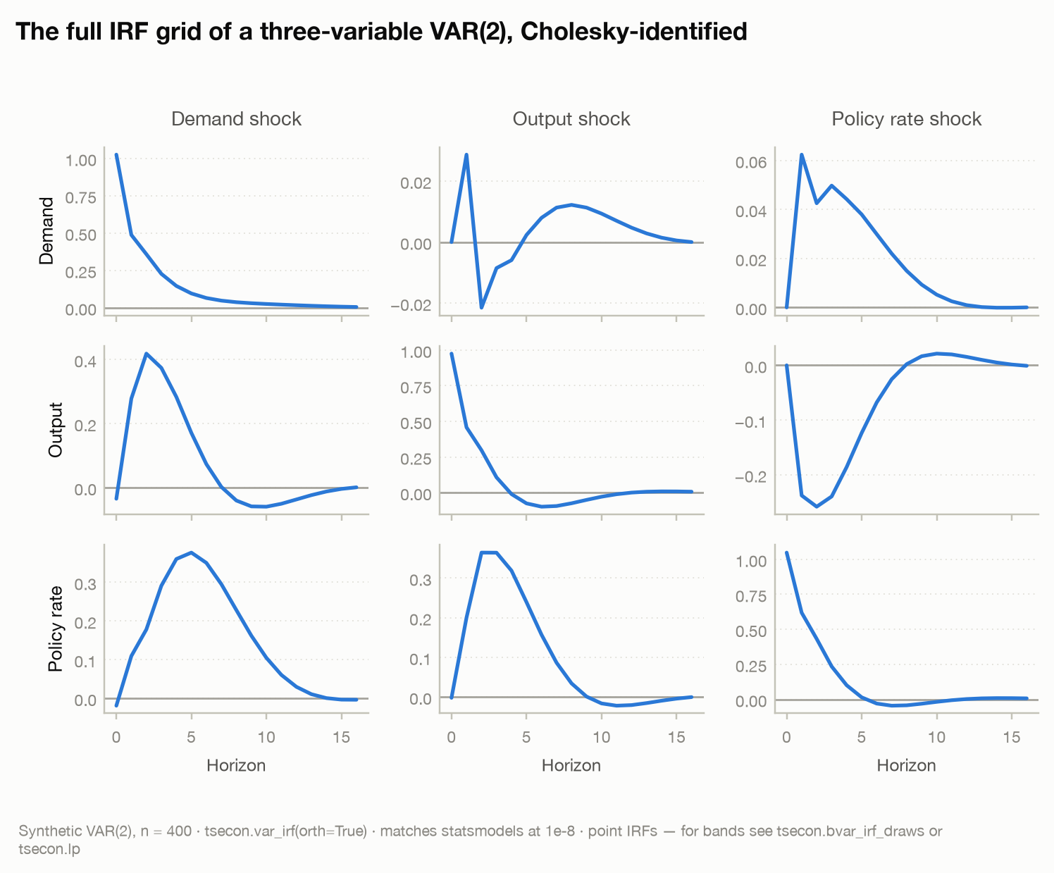
Chapter 16 takes this comparison head to head with measured numbers: where the two finite-sample estimates coincide exactly (and where the popular claim that they do is wrong), the LPW bias-variance trade-off reproduced on a seeded Monte Carlo, and the decision rule that follows.
The practical upshot of the equivalence result: fit both and overlay them. When LP and VAR IRFs from the same specification diverge, that divergence is information — usually a sign the VAR's lag length is too short — not a reason to pick your favorite. The roadmap module makes this dual reporting a single call.
⚠ Common mistake — treating LP/VAR divergence as one method being "broken." They are two estimators of one estimand. Divergence at long horizons is the expected signature of VAR extrapolation bias meeting LP noise, and its pattern is a useful specification diagnostic. Reporting only whichever line looks better is the field's version of p-hacking.
Inference done right
Here is where existing tools fail and where the most has changed since 2005. Getting the point estimates right is easy; getting the standard errors right is the hard part, because those MA(\(h\)) errors violate the OLS independence assumption at every horizon past zero.
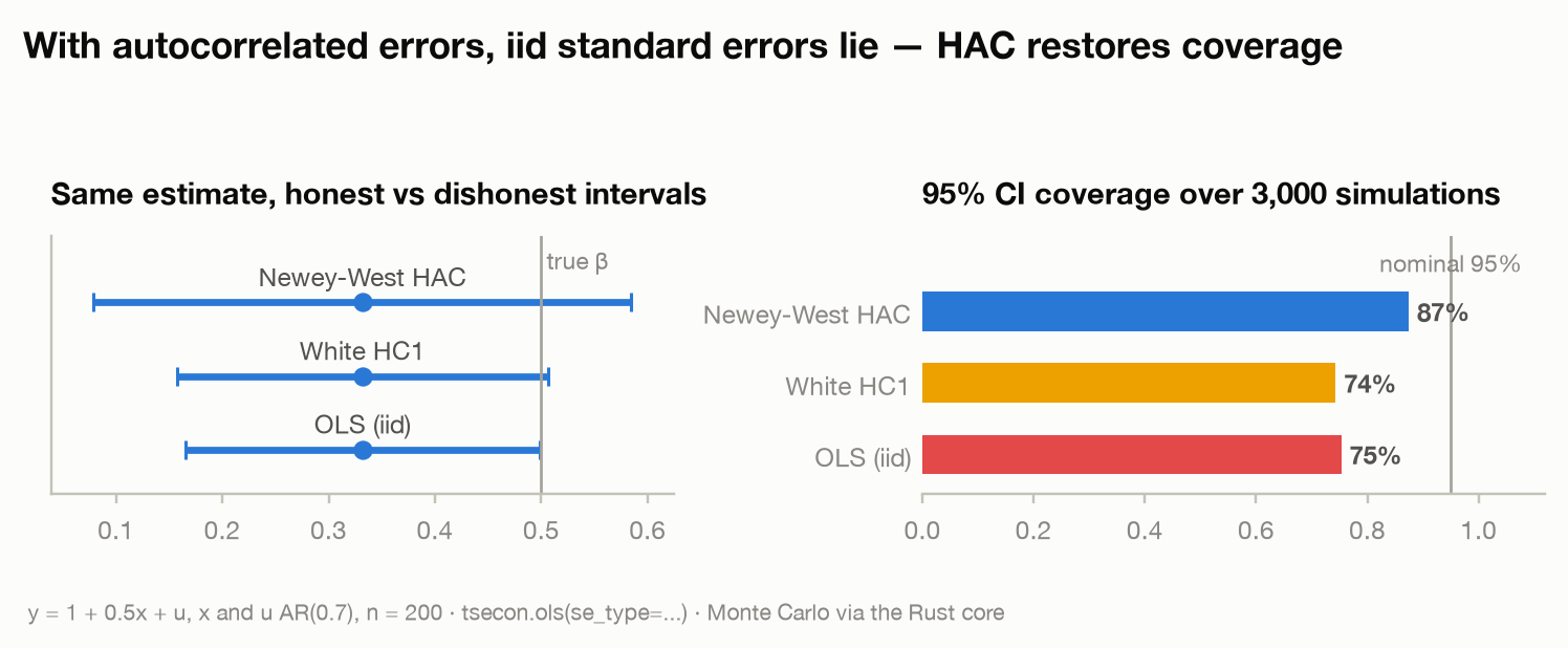
The old default: per-horizon HAC. Since the errors are serially correlated up to order \(h\), the traditional fix is Newey-West (HAC) standard errors, horizon by horizon, with a bandwidth that grows with \(h\) — you saw it in the first code block. This works asymptotically, but it has known problems: HAC estimators undercover in small samples (the true 95% interval covers less than 95% of the time), the distortion worsens as the bandwidth grows — which it must, since the error order grows with \(h\) — and the popular folklore bandwidth-equals-\(h\) rule is exactly that: folklore. The gallery's robust-standard-errors figure shows the undercoverage phenomenon in its simplest form — nominal 95% intervals covering ~75% under naive standard errors, with Newey-West closing most but not all of the gap:
The new default: lag augmentation. Montiel Olea and Plagborg-Møller (2021) showed something surprising. Take the LP regression and augment it with \(p\) lags of all system variables:
where \(Y_t\) stacks the outcome, the impulse, and any other system variables. If the impulse \(\varepsilon_t\) is innovation-like — unpredictable from the past, as a properly identified shock should be — then the part of the regression score attached to \(\beta_h\) becomes approximately a martingale difference sequence: serially uncorrelated, despite the MA(\(h\)) errors. Plain heteroskedasticity-robust (Eicker-Huber-White) standard errors are then valid. No HAC, no bandwidth choice at all.
Better still, the result is uniform: it holds whether the data are mildly persistent or have an exact unit root, and it holds at horizons that are a nontrivial fraction of the sample — precisely the territory where HAC-based LP inference is known to break down. Simpler and more robust. This is why tsecon.lp makes lag-augmented LP with robust standard errors its default: pass no se and you get "lag_augmented", with HAC the explicit fallback. There is one carve-out, where the argument itself fails: under cumulative="both" the regressor is sum_(j=0..h) shock_(t+j), so nearby base times share future shocks that no past-lag augmentation can project out, the score is not a martingale difference, and lag-augmented HC1 intervals collapse (the audit measured 0.507 coverage at a nominal 95%, h=12, flat in T). For that mode tsecon.lp and tsecon.lp_state default to HAC instead, stamp the choice in the returned se_method, and refuse an explicit se="lag_augmented" with an error that says why.
The lag-augmented version of our example, using today's API:
p = 2                                    # augmentation lags
irf_la = np.zeros(H + 1)
se_la = np.zeros(H + 1)
for h in range(H + 1):
    t = np.arange(p, T - h)              # t where all lags and leads exist
    yh   = y[t + h]
    s    = eps[t]
    lags = np.column_stack([y[t - j] for j in range(1, p + 1)])
    X = np.column_stack([np.ones(t.size), s, lags])
    r = tsecon.ols(yh, X, se_type="hc1")   # plain robust SEs -- no HAC needed
    irf_la[h], se_la[h] = r["params"][1], r["bse"][1]
The only changes from the first loop: extra lags in the design matrix, and se_type="hc1" instead of "hac". That swap is the entire modern inference upgrade. Comparing the two ladders of standard errors on our synthetic data:
hs = [0, 4, 12, 20]
print(np.round(se[hs], 3))     # per-horizon HAC:   [0.028 0.091 0.072 0.072]
print(np.round(se_la[hs], 3))  # lag-augmented EHW: [0.028 0.081 0.081 0.078]
Two things to notice. Both ladders grow with the horizon — at impact the regression explains almost everything, while at horizon 20 twenty periods of intervening shocks sit in the error, so uncertainty about long-horizon responses is intrinsically larger. And in this easy DGP — stationary, moderate persistence, 400 observations — the two ladders nearly coincide. That is expected: the case for lag augmentation is not that it gives different answers in easy problems, but that it keeps giving valid answers in the hard ones (persistence near or at a unit root, horizons that are a sizable fraction of the sample) where HAC-based intervals are known to undercover badly. You pay nothing in the easy case and you are protected in the hard case, which is what a good default looks like.
When samples are small: the bootstrap, done carefully. Below a couple hundred observations, even good asymptotic approximations strain, and the bootstrap becomes attractive — but LP is a minefield for naive resampling. Resampling per-horizon residuals independently is flat-out invalid: the residuals are dependent both within a horizon (the MA(\(h\)) structure) and across horizons (they share intervening shocks). The schemes that work are the wild bootstrap on the lag-augmented regression's scores — the natural partner of the lag-augmented default, per Montiel Olea and Plagborg-Møller (2021) — and the moving-block bootstrap on entire data tuples \((y_{t+h}, s_t, w_t)\), which preserves dependence by resampling contiguous chunks. In either case, use studentized (percentile-t) intervals: Kilian and Kim (2011) showed plain percentile intervals for LP have poor coverage. You can experiment with the block machinery today via tsecon.bootstrap_indices and tsecon.optimal_block_length; the LP-specific schemes, wired to reproducible parallel RNG so thousands of replications take seconds, are what the roadmap module adds.
⚠ Common mistake — lag augmentation is not a free pass. The EHW-validity result requires the impulse regressor to be innovation-like. If your "impulse" is a persistent observable — the level of the interest rate, an oil price — rather than an unforecastable shock, the score is not a martingale difference and HAC standard errors are still required. The inference mode must match what the impulse is. tsecon's LP module makes this an explicit, validated API choice rather than a silent default; when hand-rolling, you have to police it yourself. And in the other direction: never pair a small-bandwidth HAC estimator with long horizons on near-unit-root data and trust the bands — that is the configuration the Monte Carlo literature shows failing worst.
Beyond pointwise: joint and simultaneous bands
Every IRF plot you have ever seen has a shaded band around the line. Almost all of them are pointwise 95% intervals: at each horizon separately, the interval covers the true response 95% of the time. But readers never use them pointwise — they ask "is the response significant over horizons 4 through 16?" or "is the whole path different from zero?" Those are joint statements across 13 or 21 horizons, and the probability that a true IRF escapes at least one of 21 pointwise intervals is far more than 5%. Pointwise bands systematically overstate joint significance.
The honest object is a simultaneous confidence band: a band that contains the entire true IRF path with 95% probability. The workhorse construction is the sup-t band (Montiel Olea and Plagborg-Møller 2019): estimate the joint covariance of the whole IRF vector \((\hat\beta_0, \dots, \hat\beta_H)\) — including the cross-horizon correlations induced by overlapping samples — then simulate the distribution of the maximum absolute t-statistic across horizons and widen every interval by that common critical value instead of 1.96. The result is wider than pointwise (it must be) but much narrower than a Bonferroni correction, because it exploits the strong positive correlation between adjacent horizons' estimates.
The prerequisite is the joint cross-horizon covariance matrix, which requires estimating all horizons as one stacked system rather than \(H+1\) unrelated regressions. That machinery now exists: lp_irf_cov in the tsecon-lp crate builds the full cross-horizon matrix from the Frisch-Waugh-Lovell influence function, and band="sup-t" on lp uses it. It is a Rust-side object, not a Python callable — you reach it through band=, which also reports cov_se_max_rel_diff, the largest relative gap between that covariance's own \(\sqrt{\mathrm{diag}}\) and the reported se. It is first-class internally precisely so that sup-t bands, path Wald tests ("is the IRF zero at all horizons?"), and multiplier delta methods all fall out of it; the latter two remain roadmap. Computing per-horizon standard errors and pretending horizons are independent produces bands that are wrong in both width and shape.
A useful companion object is the significance band (Inoue, Jordà, and Kuersteiner 2023): instead of a band around the estimate, construct the band around zero that the estimated IRF would stay inside if the true response were nil, accounting for serial dependence under that null. It answers a different question — "is there any response at all?" versus the confidence band's "what responses are consistent with the data?" — exactly the way the Bartlett bands on an ACF plot work. When a referee asks whether your IRF is distinguishable from no effect, this is the clean answer; it comes nearly for free once the joint covariance exists.
⚠ Common mistake — reading pointwise bands as joint statements. "The IRF is significant from quarter 2 to quarter 10" is a claim about 9 horizons at once; pointwise bands do not license it. Nearly every published LP paper commits this quietly. If your conclusion is about a stretch of the IRF or its shape, you need simultaneous bands — and if a result survives only under pointwise bands, that is worth knowing before a referee finds out.
LP-IV and fiscal multipliers
Now the running example the whole modern fiscal literature is built on. Question: if the government spends an extra dollar, how many dollars of GDP do we get? The obstacle: government spending is not randomly assigned — it responds to the state of the economy — so regressing output on spending confuses cause and effect.
Ramey and Zubairy (2018) attack this with an instrument: military news — narrative-identified changes in expected defense spending driven by geopolitical events (wars, threats), which move government spending for reasons plausibly unrelated to the current business cycle. This is LP-IV: at each horizon, a two-stage least squares regression where the endogenous impulse (spending) is instrumented by the external shock (news). Writing \(\tilde{\cdot}\) for variables residualized on the controls, the horizon-\(h\) estimator is
with \(z_t\) the instrument, \(x_t\) the endogenous impulse, \(y_{t+h}\) the shifted outcome. Validity requires more than the textbook IV conditions: Stock and Watson (2018) show LP-IV needs lead-lag exogeneity — the instrument must be uncorrelated with past and future structural shocks, not just contemporaneous ones — which in practice means the control set must be rich enough to absorb any autocorrelation in the instrument, and must be identical across both stages. A per-horizon first-stage effective F statistic (in the HAC-robust form of Montiel Olea and Pflueger) is the standard weak-instrument diagnostic; narrative instruments are frequently weak, so this is not optional. When the F is uncomfortably low, the honest reporting object is a weak-instrument-robust Anderson-Rubin confidence set rather than a point estimate with fictional precision — more on that in the frontier section.
The same design runs the monetary literature. Gertler and Karadi (2015) instrument the policy rate with high-frequency surprises — the jump in federal funds futures prices in a 30-minute window around FOMC announcements, too narrow a window for anything but the policy news itself to move prices. Swap the instrument and the endogenous impulse, keep every line of the LP-IV machinery, and the fiscal toolkit becomes a monetary one. This plug-compatibility across identification schemes is a large part of why LP displaced bespoke structural models as the default reporting device.
Cumulative multipliers. A fiscal multiplier is not a single-horizon object — "the effect of a dollar" should count all the output gained over, say, four years, per dollar of spending over those four years. The modern standard estimates this in one step: regress cumulated output on cumulated spending, instrumented by the shock,
so the coefficient \(\mathcal{M}_h\) is the horizon-\(h\) multiplier, with correct IV inference built in. Ramey and Zubairy's headline number — a linear multiplier of roughly 0.6 to 0.7 at two-to-four-year horizons, below the "spend a dollar, get a dollar" threshold of 1 — comes from exactly this construction on 125+ years of US quarterly data, and it is the single most important validation target for tsecon's LP module.
One unglamorous detail that changes headline numbers: units. A multiplier should be "dollars of output per dollar of spending," but the natural regression variables are log GDP and log spending, whose coefficient is an elasticity — and converting an elasticity to a multiplier requires multiplying by the sample-average GDP/spending ratio, a number around 5 for the US, applied ex post and frozen at one value even though the ratio moves over a century of data. The Gordon-Krenn transformation avoids this: divide both output and spending by an estimate of trend GDP before running the LP, so both variables are already in "percent of trend GDP" units and the coefficient is a multiplier directly. Ramey and Zubairy use exactly this, and the roadmap module treats the transformation as a first-class option rather than a preprocessing chore.
Per-horizon 2SLS ships today as tsecon.lp_iv: pass the outcome, the endogenous impulse, and the instrument, and it returns per-horizon IRFs, standard errors, and a first-stage effective F. Two cumulative objects come out of this machinery, and conflating them is the classic way to report a wrong multiplier:
- The cumulative IRF.
lp_iv(..., cumulative=True)cumulates only the outcome: the horizon-\(h\) coefficient is \(\sum_{j=0}^{h} y_{t+j}\) per unit of contemporaneous spending. Because the numerator keeps accumulating while the denominator stays a one-period impulse, this number grows with the horizon by construction. It is a perfectly good summary of the output path; it is not a multiplier. - The integral multiplier.
tsecon.lp_multiplierruns the one-step Ramey-Zubairy regression displayed above — cumulated output on cumulated spending, instrumented by the shock — so both sides accumulate over the same window and \(\mathcal{M}_h\) is cumulated output per unit of cumulated spending, estimated as a single 2SLS parameter with honest HAC standard errors on that number (not a ratio of two separately estimated responses with a delta method bolted on).
Here are both on a synthetic fiscal system where a confounder moves both spending and output, so naive OLS overstates the multiplier while the news instrument recovers it:
rng = np.random.default_rng(7)
T = 400
military_news = rng.standard_normal(T)               # exogenous instrument (news shock)
confounder    = rng.standard_normal(T)               # moves both spending and output
spending = np.zeros(T)                               # endogenous impulse
output   = np.zeros(T)                               # outcome
for t in range(1, T):
    spending[t] = 0.5 * spending[t - 1] + military_news[t] + 0.4 * confounder[t]
    output[t]   = 0.5 * output[t - 1]   + 0.6 * spending[t] + confounder[t]

# Naive OLS confuses cause and effect: the confounder inflates the slope.
biased = tsecon.ols(output[1:], np.column_stack([np.ones(T - 1), spending[1:]]))
print(round(biased["params"][1], 2))                 # 1.14 -- far above the true 0.6

# LP-IV instruments spending with the news shock at every horizon.
res = tsecon.lp_iv(output, spending, military_news, horizons=20, n_lag_controls=4)
print(round(res["irf"][0], 2))                        # 0.55 -- recovers the true impact effect of 0.6
print(round(res["first_stage_f"][0], 0))              # 1588 -- news is a strong instrument

# cumulative=True cumulates ONLY the outcome: a cumulative IRF, not a multiplier.
cum_resp = tsecon.lp_iv(output, spending, military_news,
                        horizons=20, n_lag_controls=4, cumulative=True)
print(round(cum_resp["irf"][8], 2))                   # 2.91 -- cumulated output per unit of impact spending

# lp_multiplier cumulates BOTH sides: the one-step Ramey-Zubairy integral multiplier.
mult = tsecon.lp_multiplier(output, spending, military_news,
                            horizons=20, n_lag_controls=4)
print(round(mult["multiplier"][8], 2))                # 1.33 -- the DGP's true integral multiplier here is ~1.19
print(round(mult["se"][8], 2))                        # 0.14 -- HAC SE on the multiplier coefficient itself
print(round(mult["first_stage_f"][8], 0))             # 53 -- cumulated-impulse first stage, still strong
Read the contrast: at two years the cumulative IRF says 2.91 and is still climbing (it must — its denominator is a one-period impulse), while the integral multiplier says 1.33 ± 0.14, sitting on the DGP's true value — cumulated output over cumulated spending converges to \(0.6/(1-0.5) = 1.2\), and equals 1.19 at \(h = 8\). Only the second number answers "how many dollars of output per dollar of spending." lp_multiplier also returns the two reduced-form legs, cumulative_outcome and cumulative_impulse, whose ratio reproduces the multiplier by the just-identified IV algebra — useful for plotting, but the headline coefficient and its standard error come from the one-step regression.
The first_stage_f ladder — reported by both estimators — is the Montiel Olea-Pflueger effective F, horizon by horizon; a value below the rule-of-thumb 10 is the signal to switch from a point estimate to a weak-instrument-robust Anderson-Rubin set. sup-t simultaneous bands now ship for lp and smooth_lp via band="sup-t". lp_iv, lp_multiplier and lp_state have no cross-horizon covariance yet, so they get Šidák/Bonferroni only and refuse sup-t with an error rather than approximating one. Anderson-Rubin sets for LP-IV remain on the roadmap.
⚠ Common mistake — the ratio-of-IRFs multiplier. It is tempting to estimate the cumulative output IRF and the cumulative spending IRF separately and report their ratio, delta-method standard errors attached. That is a different estimator from the one-step IV regression, and the two can differ materially in finite samples — the one-step version is the standard for good reason (Ramey and Zubairy 2018).
lp_multiplierfollows suit: the two cumulated legs come back as a labeled comparison, never as the headline number.
State dependence, panels, and other extensions
The reason LP won the applied-macro market is that each extension below is just a variation on a regression — no new estimation theory required to run them (the theory shows up in the caveats).
State-dependent LP. Is the fiscal multiplier bigger in recessions, when idle resources make crowding-out weaker? Interact everything — impulse, controls, intercept — with a lagged state indicator \(I_{t-1}\) (recession/expansion, high/low slack):
giving one IRF per regime. The smooth-transition variant (Auerbach and Gorodnichenko 2012) replaces the on/off dummy with a logistic weight \(F(z_t) = \exp(-\gamma z_t)/(1 + \exp(-\gamma z_t))\) on a standardized state variable \(z_t\), so the IRF varies continuously with the depth of the recession; Auerbach and Gorodnichenko calibrate \(\gamma = 1.5\). Ramey and Zubairy's state-dependent results combine the dummy-interaction design with the one-step IV multiplier, and are the module's headline validation target. Their substantive finding is worth knowing because it reversed the field's prior: where Auerbach and Gorodnichenko had reported recession multipliers well above 1, Ramey and Zubairy — with a longer sample, the one-step multiplier estimator, and careful attention to the state variable's construction — find little evidence that multipliers exceed 1 even in high-slack states. Methodological choices this chapter has been cataloging (estimator, sample convention, state timing) are exactly what separates the two conclusions.
tsecon.lp_state runs the dummy-interaction design today: the impulse and controls are interacted with the lagged state indicator, so the regime is predetermined, and it returns one IRF per regime. On a synthetic system whose impact response is deliberately larger in recessions:
rng = np.random.default_rng(11)
Ts = 400
shock = rng.standard_normal(Ts)                            # identified shock
recession = (rng.standard_normal(Ts) > 0.3).astype(float)  # predetermined 0/1 state
y = np.zeros(Ts)
for t in range(1, Ts):
    impact = 1.4 if recession[t - 1] else 0.5              # bigger impact in recessions
    y[t] = 0.5 * y[t - 1] + impact * shock[t] + rng.standard_normal()

res = tsecon.lp_state(y, shock, recession, horizons=20, n_lag_controls=4)
print(round(res["irf_state1"][0], 2))                     # 1.36 -- impact response, recession
print(round(res["irf_state0"][0], 2))                     # 0.39 -- impact response, expansion
The binary indicator is the design Ramey and Zubairy use. The smooth-transition (logistic) weighting of Auerbach-Gorodnichenko — which lets the IRF vary continuously with the depth of the recession rather than an on/off switch — is still on the roadmap.
⚠ Common mistake — a state variable that responds to the shock. The state must be predetermined: use \(I_{t-1}\), not \(I_t\). But even lagging does not fully solve the deeper problem identified by Gonçalves, Herrera, Kilian, and Pesavento: if the shock itself can move the economy across regimes within the response horizon, the regime-specific "IRF" no longer means what you think it means — the estimand changes. Relatedly, building the state from a centered moving average or two-sided filter smuggles future information into the regime classification (the standard critique of Auerbach-Gorodnichenko's original state variable). tsecon's implementation emits diagnostics for both traps.
Panel LP. With many countries, firms, or households, run the LP within-units: unit fixed effects absorb permanent differences, time effects absorb common shocks, and the standard errors must respect the panel structure — clustered by unit, two-way, or Driscoll-Kraay when cross-sectional dependence is pervasive (which in macro panels it always is). This is the engine of the Jordà-Schularick-Taylor macrohistory literature: what follows credit booms, across 17 countries and 150 years, is a panel LP question. Watch for two panel-specific pathologies. Nickell bias — the familiar dynamic-panel bias from combining fixed effects with lagged outcomes — does not stay \(O(1/T)\) in LP but grows with the horizon (effectively \(O(h/T)\)), dangerous exactly when your panel is short and your horizons long. And unbalanced panels develop different gaps at each horizon once outcomes are shifted \(h\) periods, so the effective sample quietly changes shape across the IRF. All of this is tsecon.panel_lp, with Driscoll-Kraay the default se_type and two half-panel jackknives for the Nickell problem: bias_correction="jackknife" (Dhaene-Jochmans, point estimates only) and bias_correction="spj" (Mei-Sheng-Shi split-panel, which recomputes the standard errors for the corrected estimator). At short \(T\) prefer "spj" — the docstring carries the measured coverage: the DJ jackknife's reported se runs ~36% below the true sd at \(T=60\), dropping 95% coverage to 0.80, and only catches up around \(T \approx 240\).
LP-DiD. Difference-in-differences event studies are LPs in disguise: regress the \(h\)-horizon change in the outcome on treatment switching. Dube, Girardi, Jordà, and Taylor (2023) formalize this and add the crucial clean-control condition — compare switchers only to not-yet-treated or never-treated units — which sidesteps the negative-weighting pathologies that plague two-way-fixed-effects event studies under staggered adoption. The LP framing also makes pre-trend checks natural: run the same regressions at negative horizons (\(h < 0\)), where a well-identified design should show flat responses before treatment. If you know the modern DiD literature, LP-DiD is the time-series native's route to the same destination — and it ships as tsecon.lp_did(outcome, treatment, ...), with the clean-control rule built in (not-yet-treated under absorbing=True, unchanged-for-nonabsorbing_lag when treatment can revert, never-treated under never_treated_only=True), pre-treatment horizons back to -pre_window for the pre-trend check, entity-clustered SEs in the authors' fixest/reghdfe convention, and reweight=True for the equally-weighted ATT instead of OLS's variance-weighted one. It returns n_switchers per horizon alongside coef/se, and you should read it: the clean sample shrinks as \(|h|\) grows.
Smoothing the jagged path: smooth local projections
Raw LP estimates are jagged because each horizon is estimated separately — but true IRFs are smooth, and readers will interpret every wiggle ("the effect dies at quarter 9 and revives at quarter 11") even when the wiggles are pure noise. Barnichon and Brownlees (2019) attack the jaggedness at its source: instead of \(H+1\) unrelated coefficients, write the IRF as a smooth function of the horizon — a B-spline expansion \(\beta_h = \sum_k \theta_k B_k(h)\) — and estimate all horizons jointly, with a ridge penalty on the second differences of the basis coefficients that shrinks the path toward a straight line:
Information now flows across neighboring horizons — the horizon-9 estimate borrows strength from horizons 8 and 10 — and variance drops sharply at the price of a little smoothing bias. That is the same bias-variance dial as LP-versus-VAR, but turned continuously by a single knob \(\lambda\) rather than by switching estimators.
tsecon.smooth_lp implements this with two design decisions worth knowing. First, the \(\lambda = 0\) anchor: with the penalty off, the joint estimator collapses exactly to the per-horizon lp(se="hac") point estimates — machine precision, pinned in the test suite — so smooth LP is never a different model, only the same LP with its horizons asked to agree. Second, the cross-validation is blocked: lam="cv" tunes \(\lambda\) by leave-one-block-out CV over contiguous horizon-blocks with a dependence buffer of horizons + n_lag_controls periods around each held-out block, because ordinary k-fold leaks the MA(\(h\)) overlap across folds and systematically undersmooths. On the chapter's running DGP (where the truth is \(0.7^h\)):
rng = np.random.default_rng(42)                  # rebuild the chapter's opening DGP
T, H, phi = 400, 20, 0.7
eps, eta = rng.standard_normal(T), rng.standard_normal(T)
y = np.zeros(T)
for t in range(1, T):
    y[t] = phi * y[t - 1] + eps[t] + 0.5 * eta[t]

sm = tsecon.smooth_lp(y, eps, horizons=H, n_lag_controls=1, lam="cv")
sm["lambda_used"]                                # 538.2 — chosen by blocked CV on a log grid
                                                 # (the default grid is scale-relative: anchored to
                                                 # X'X, so this choice is invariant to the units
                                                 # of y and eps; see the model card)

true = phi ** np.arange(H + 1)
print(np.round(np.array(sm["irf_raw"])[:6], 2))  # [0.98 0.74 0.49 0.3  0.24 0.19]  per-horizon LP
print(np.round(np.array(sm["irf"])[:6], 2))      # [0.94 0.72 0.52 0.36 0.24 0.16]  smoothed
print(np.round(true[:6], 2))                     # [1.   0.7  0.49 0.34 0.24 0.17]

rmse = lambda a: float(np.sqrt(np.mean((np.array(a) - true) ** 2)))
print(round(rmse(sm["irf_raw"]), 3), round(rmse(sm["irf"]), 3))   # 0.068 -> 0.055 against the truth
The smoothed path gives up a little at impact (0.94 versus the true 1.0 — shrinkage bias, exactly where the IRF bends fastest) and pays it back everywhere else: RMSE against the true path drops from 0.068 to 0.055, and the long-horizon wiggles that invite over-interpretation are gone. The anchor is checkable in one line:
sm0 = tsecon.smooth_lp(y, eps, horizons=H, n_lag_controls=1, lam=0.0)
lp0 = tsecon.lp(y, eps, horizons=H, n_lag_controls=1, se="hac")
np.abs(np.array(sm0["irf"]) - np.array(lp0["irf"])).max()   # 3.0e-13 — same estimator, penalty off
The returned se is a delta method through the basis over a stacked Bartlett-HAC sandwich — and it is honest about what it is: it conditions on \(\lambda\) (even a cross-validated one) and describes the penalized estimator's own sampling variability, not the shrinkage bias. That is the "post-shrinkage inference is unsolved" caveat from the frontier section made concrete; irf_raw/se_raw always come back alongside, so the unshrunk comparison is never more than one plot away. Both the B-spline basis (against scipy BSpline.design_matrix) and the full estimator (against NumPy normal equations) are golden-tested; see the local-projections model card for the contract.
⚠ Common mistake — reporting only the smoothed path. Smoothing is a presentation and an estimation choice, and \(\lambda\) is a researcher degree of freedom. Show
irf_rawnext toirf(or at least reportlambda_usedand the CV grid), and be suspicious of any smoothed IRF whose economically important feature — a hump, a sign flip — is absent from the raw path. If the feature only exists after smoothing, the penalty put it there.
When the shock is a curve: functional local projections
Every LP so far took a scalar impulse. But some shocks arrive as entire curves: an FOMC announcement moves the whole yield curve — 3 months to 30 years — in one afternoon, and an OPEC surprise moves the whole oil futures strip. Collapsing that object to one number (the 2-year rate, the front-month future) throws away exactly the information that distinguishes a level shock from a twist — and those can have very different effects on the economy. Inoue and Rossi (2021) formalize the alternative: treat the curve itself as the shock, and estimate the response of an outcome to an arbitrary shift of the whole curve.
The machinery is a two-step. First, compress the \(T \times M\) panel of observed curves with functional principal components: functional_pca demeans, eigendecomposes the \(M \times M\) covariance, and returns the leading eigenfunctions (the shapes: level, slope, curvature in yield-curve applications), their scores (how much of each shape each period's curve contains), and explained shares — numpy-eigh-validated, with a documented sign convention (each eigenfunction's largest-magnitude entry is positive). Second, run a joint LP of the outcome on all \(K\) scores at once (flp): per horizon, \(y_{t+h}\) on the \(K\) scores, a constant, and lags of \(y\), with Newey-West HAC — jointly, because the response to any curve scenario mixes all the betas, so you need their joint covariance, not \(K\) separate regressions.
Then any scenario you can draw is a linear combination: a curve shift \(\delta(\cdot)\) has score-weights \(w_k = \langle \phi_k, \delta \rangle\), and the response of \(y\) is \(w'\beta_h\) with standard error \(\sqrt{w' \,\mathrm{Cov}_h\, w}\). flp_scenario does the whole pipeline in one call. On a synthetic yield-curve panel driven by a level factor and a short-end slope factor, where the outcome responds \(-0.8\) to level and \(+0.5\) to slope:
rng = np.random.default_rng(3)
T, M = 400, 8
grid = np.array([0.25, 0.5, 1, 2, 3, 5, 7, 10])            # maturities in years
level = np.ones(M)                                          # parallel-shift loading
slope = np.exp(-grid / 2.0) - np.exp(-grid / 2.0).mean()    # short-end twist, demeaned
L, S = rng.standard_normal(T), rng.standard_normal(T)
curves = np.outer(L, level) + np.outer(S, slope) + 0.05 * rng.standard_normal((T, M))

yy = np.zeros(T)
for t in range(1, T):
    yy[t] = 0.5 * yy[t - 1] - 0.8 * L[t] + 0.5 * S[t] + rng.standard_normal()

fp = tsecon.functional_pca(curves, n_factors=2)
np.round(np.array(fp["explained"]), 3)          # [0.907 0.091] — two shapes carry 99.8%
np.round(np.array(fp["eigenfunctions"][0]), 2)  # [0.34 .. 0.36] — flat: the level shape
np.round(np.array(fp["eigenfunctions"][1]), 2)  # [0.57 0.45 .. -0.39] — the slope shape

# The response of yy to the WHOLE curve shifting up in parallel by 1:
par = tsecon.flp_scenario(yy, curves, np.ones(M), n_factors=2, horizons=8, n_lag_controls=2)
print(np.round(np.array(par["response"]), 2))   # [-0.82 -0.41 -0.18 -0.01 -0.02 -0.01  0.01 -0.04 -0.  ]
print(np.round(np.array(par["se"])[:3], 2))     # [0.05 0.06 0.07]

# The response to a pure short-end steepening of the same size:
tw = tsecon.flp_scenario(yy, curves, slope, n_factors=2, horizons=8, n_lag_controls=2)
print(np.round(np.array(tw["response"])[:3], 2))   # [0.51 0.24 0.09] — opposite SIGN
The truth for the parallel shift is \(-0.8 \times 0.5^h = [-0.8, -0.4, -0.2, \dots]\), and the estimate sits on it. But the punchline is the second scenario: a steepening of the same magnitude moves the outcome in the opposite direction (\(+0.51\) on impact). A scalar-shock LP on any single point of the curve would have averaged those two responses into something misleading about both — which is the entire case for treating the curve as the object.
The internal consistency is checkable, and test-pinned: feed the \(j\)-th eigenfunction itself in as the scenario and the response must reproduce the \(j\)-th column of the joint FLP betas exactly (\(w\) becomes the \(j\)-th unit vector):
res = tsecon.flp(yy, np.array(fp["scores"]), horizons=8, n_lag_controls=2)
sc  = tsecon.flp_scenario(yy, curves, np.array(fp["eigenfunctions"][0]),
                          n_factors=2, horizons=8, n_lag_controls=2)
np.abs(np.array(sc["response"]) - np.array(res["betas"])[:, 0]).max()   # 5.6e-17
⚠ Common mistake — trusting
flp's per-score standard errors as if the scores were observed. The scores arefunctional_pcaestimates, i.e. generated regressors, and the HAC sandwich inflpconditions on them as if they were data — the same two-step hazard flagged for FAVAR factors in chapter 7 and for the dynamic Nelson-Siegel two-step in chapter 15. Measured: the per-elementseruns about 0.66 of the true sampling sd, flat over a 16× range of \(T\) (so it is inconsistency, not a small sample — coverage ≈ 0.80 against a nominal 0.95), and it worsens as the curve panel's signal-to-noise falls; on the model card's own worked example the second score'sseis one-fifth of the truth. Scores you supply from outside are real data and theseis then correct. The route that survives estimation of the basis is the one this section already reports:flp_scenario's \(w'\beta\) contrast is algebraically invariant to rotations of the estimated eigenfunctions (rotate \(\hat\Phi\) and the weights rotate to match), so quote scenario responses and theirse, not raw per-score betas — the functional-shocks model card carries the measured numbers.
There is also a VAR route to the same question: fvar_scenario fits a VAR to [scores, y] (scores ordered first), identifies with a Cholesky factorization, sets the score innovation to \(w = \phi'\delta\), and reads the outcome response off the orthogonalized IRFs. It buys the usual VAR smoothness at the usual VAR price plus one more assumption worth saying out loud: the recursive ordering sets the outcome's own contemporaneous structural shock to zero in the scenario, so the impact response of \(y\) is an identification choice, not an estimate. The FLP route is the robust default; the FVAR route is the cross-check, per the dual-reporting discipline of this chapter. Contracts, the sign convention, and validation for the whole family live in the functional-shocks model card.
⚠ Common mistake — reading eigenfunction responses as economics. The \(K\) score paths from
flpare responses to statistical shapes: whatever directions happen to dominate the sample covariance of the curves, in units set by the normalization \(\|\phi_k\| = 1\). They are not "the effect of monetary policy" until you map an economically meaningful scenario — a parallel 100bp hike, a 2s10s flattening, the announcement-day curve change itself — throughflp_scenario, which is why the scenario interface, not the raw betas, is the reporting object. And mind the truncation:explainedtells you how much of the curves' variation your \(K\) factors carry; a scenario \(\delta\) that loads heavily on discarded shapes (\(w \approx 0\) despite \(\delta \neq 0\)) is answered with "no response" not because the economy is indifferent but because the basis cannot see it.
The frontier
The LP literature is one of the most active in econometrics; here is the current edge. Most of it sits in the roadmap module's upper tiers — but not all, as the last item records.
Efficiency without a VAR's bias. The MA(\(h\)) error structure is known, which OLS ignores. Lusompa (2023) exploits it with a recursive GLS transformation using earlier-horizon estimates, recovering large efficiency gains; inference must be by wild bootstrap because estimation error propagates across horizons. Bayesian LP (Ferreira, Miranda-Agrippino, and Ricco; Tanaka 2020) places VAR-based priors on the IRF path, landing the estimator on the LP-VAR bias-variance frontier by choice rather than accident. And Li, Plagborg-Møller, and Wolf (2024) show penalized LP-VAR averaging dominates both endpoints in MSE — with the honest caveat that post-shrinkage inference remains an unsolved problem: nobody knows how to build fully honest confidence bands after data-driven shrinkage, so these ship with bootstrap bands and loud warnings.
Small-sample honesty. LP point estimates carry a finite-sample bias analogous to the classic AR-coefficient bias, growing with horizon and persistence; Herbst and Johannsen (2024) derive a feasible analytical correction. On the bootstrap side, Kilian and Kim (2011) showed percentile intervals for LP have poor coverage — studentized (percentile-t) intervals on block or wild resampling are the standard, and naive iid residual resampling is simply invalid given the dependence within and across horizons.
Why LP defaults won the argument. Montiel Olea, Plagborg-Møller, Qian, and Wolf (2024) — the memorably titled "Unpleasant VARithmetic" paper — show lag-augmented LP is doubly robust to misspecification in a sense VARs cannot match: VAR bias does not vanish even as you widen the bands. This is the intellectual foundation under the library's lag-augmented default.
Frontier variants — two shipped, the rest awaiting anyone's implementation. Two items on this list have already crossed over into the library: smooth LP (the Barnichon-Brownlees estimator of the section above) and quantile LP — how a shock moves the tails of the outcome distribution rather than its mean, the dynamic engine behind growth-at-risk (Adrian, Boyarchenko, and Giannone 2019). tsecon.quantile_lp(y, shock, taus, horizons, n_lag_controls) runs the check-loss analogue of this chapter's LP at each (tau, horizon) pair with Powell-sandwich standard errors — the same design conventions as lp, the same quantile machinery as Chapter 3, and the static one-call workflow in Chapter 5's growth-at-risk section (see the quantile model card). Still genuinely unimplemented anywhere: weak-instrument-robust Anderson-Rubin confidence sets for LP-IV (which can be unbounded or disjoint — an honest API must represent that, not truncate it); time-varying LP for unstable transmission mechanisms (Inoue, Rossi, and Wang 2024); doubly-robust IPW/AIPW LP treating policy as a treatment (Angrist, Jordà, and Kuersteiner 2018); policy counterfactuals assembled from estimated IRFs (McKay and Wolf 2023); and estimand diagnostics for nonlinear LPs — Kolesár and Plagborg-Møller (2025) characterize exactly what weighted average a misspecified nonlinear LP recovers. That remainder is the roadmap module's Tier 3 and 4 territory, and the honest reason a Rust core matters — the bootstrap- and simulation-heavy inference this literature now demands is too slow in interpreted loops to be anyone's default.
Which method when
| Situation | Reach for | Because |
|---|---|---|
| Short horizons, small well-specified system, precision matters | VAR IRFs (var_irf) |
Low variance; near-equivalent to LP at small \(h\) with matched lags |
| Medium/long horizons, misspecification a live worry | Local projections | Bias does not compound with horizon; robustness is the point |
| Observed but possibly noisy shock series | LP with the shock ordered first among controls, unit-effect normalization | Equivalent to recursive identification; normalization survives classical measurement error |
| Impulse variable endogenous, external instrument available | LP-IV with effective-F diagnostics | Lead-lag exogeneity + per-horizon 2SLS is the modern identification standard |
| Fiscal (or any integral) multiplier | One-step IV on cumulated sums (lp_multiplier) |
The Ramey-Zubairy estimator; ratio-of-IRFs is a different, inferior estimator, and outcome-only cumulation (cumulative=True) is a cumulative IRF, not a multiplier |
| Persistent data and/or long horizons | Lag-augmented LP with plain robust SEs | Uniformly valid across persistence (incl. unit roots) and horizon length |
| Impulse regressor is not innovation-like | Per-horizon HAC/HAR inference | Lag augmentation's EHW validity does not apply; HAC is the honest fallback |
| Claims about a stretch of the IRF or its shape | Sup-t simultaneous bands | Pointwise bands overstate joint significance |
| Recession-vs-expansion asymmetry | State-dependent LP with a lagged state | Predetermined states limit endogeneity; check the state isn't shock-responsive |
| Staggered policy adoption in a panel | lp_did (clean controls built in; read n_switchers per horizon) |
Avoids TWFE negative-weight pathologies, and the negative horizons are the pre-trend check |
| A common shock across a short panel, long horizons | panel_lp(bias_correction="spj") |
Nickell bias grows like \(O(h/T)\) in panel LP; the split-panel jackknife corrects the points and the SEs |
| IRF too jagged to present | smooth_lp(lam="cv") |
Joint B-spline estimation with blocked CV; lam=0 collapses to per-horizon LP, and irf_raw always comes back for comparison |
| Shock moves the tails, not the mean (growth-at-risk dynamics) | quantile_lp |
Check-loss LPs per (tau, horizon); the mean IRF cannot see downside asymmetry |
| The shock is a whole curve (yield curve, futures strip) | functional_pca + flp / flp_scenario |
Level and twist scenarios can have opposite effects; any scalar summary averages them away |
| LP and VAR disagree from the same spec | Dual reporting, then more VAR lags | Divergence is a specification diagnostic, not a horse race |
What tsecon implements today
Available now in Python — the dedicated LP estimators, plus every primitive the hand-rolled LP in this chapter needs:
tsecon.lp(baseline LP:se="lag_augmented"default andse="hac"fallback,cumulativefor cumulated-outcome responses),tsecon.lp_iv(per-horizon 2SLS with the Montiel Olea-Pflueger effective F),tsecon.lp_multiplier(the one-step Ramey-Zubairy integral multiplier: cumulated outcome on cumulated instrumented impulse, HAC SEs on the multiplier itself, per-horizon effective F, and the two reduced-form legs for inspection),tsecon.lp_state(dummy-interaction state-dependent LP, per-regime IRFs),tsecon.panel_lp(fixed-effects panel LP with clustered / Driscoll-Kraay SEs,cumulative, simultaneousband=options, and the"jackknife"/"spj"Nickell-bias corrections), andtsecon.lp_did(LP-DiD with clean controls, pre-trend horizons, pooled post/pre ATTs, and entity-clustered SEs validated against the authors' reference run)tsecon.smooth_lp(Barnichon-Brownlees joint B-spline LP:lam="cv"blocked cross-validation, the machine-precisionlam=0collapse tolp(se="hac"),irf/seplusirf_raw/se_raw, scipy-BSpline-golden basis) andtsecon.quantile_lp(check-loss LPs at each (tau, horizon) with Powell-sandwich SEs — see the quantile model card)tsecon.functional_pca,tsecon.flp,tsecon.flp_scenario,tsecon.fvar_scenario— the Inoue-Rossi functional-shock family: FPCA of a curve panel, the joint score LP with per-horizoncovs, whole-curve scenario responses, and the FVAR cross-check (see the functional-shocks model card)tsecon.ols(y, X, se_type=...)with"hac"(Newey-West,maxlagscontrols the bandwidth),"hc0"/"hc1"(the EHW standard errors that lag-augmented LP calls for), and"nonrobust"; returnsparams,bse,tvaluestsecon.long_run_variance— the kernel LRV machinery under HACtsecon.var_fit,tsecon.var_irf,tsecon.var_fevd,tsecon.var_forecast— the VAR comparator for dual reportingtsecon.bootstrap_indices,tsecon.optimal_block_length,tsecon.philox_uniforms— block-bootstrap experiments with reproducible parallel RNGtsecon.adf,tsecon.kpss,tsecon.check_stationarity— the persistence pre-flight that tells you how much to worry about long-horizon inference
Every runnable block in this chapter — the two hand-rolled loops, the VAR comparison, the LP-IV cumulative-IRF-versus-integral-multiplier contrast, the state-dependent LP, the smooth LP with its \(\lambda = 0\) anchor, and the functional-shock scenarios — works against today's API.
Not yet in lp: fixed-b/EWC (HAR) inference — the modern small-sample answer where per-horizon HAC must be used, with the Student-\(t_B\) critical values that make it size-correct. Since 0.11 it is bound for plain regressions — ols(y, X, se_type="ewc") and ewc_lrv (see the robust-inference model card) — so a per-horizon LP regression you build yourself can use it, but lp and its siblings do not take it yet; LP-EWC stays on the roadmap.
Roadmap: the dedicated module (docs/roadmap/07-local-projections.md) hardens what ships today and owns what cannot reasonably be hand-rolled: path Wald tests over the joint cross-horizon covariance (the covariance and sup-t bands themselves now ship), Anderson-Rubin weak-instrument sets for LP-IV (the proxy-SVAR analogue ships as proxy_ar_sets; the LP-IV one does not), wild and block bootstrap schemes that are actually valid for LP, the smooth-transition (logistic) state-dependent variant with endogeneity diagnostics, Bayesian and GLS LP, and LP-VAR dual reporting. LP-DiD has left this list — it ships as lp_did. Its validation bar: reproduce the Ramey-Zubairy multipliers and the lpirfs/Stata reference numbers to three-plus decimals.
Further reading
- Jordà (2005), American Economic Review — the founding paper: impulse responses by per-horizon regression, and why robustness to misspecification is worth variance.
- Ramey & Zubairy (2018), Journal of Political Economy — the applied benchmark: military-news LP-IV, one-step cumulative multipliers, state dependence, 125+ years of US data.
- Stock & Watson (2018), Economic Journal — the LP-IV foundations, including the lead-lag exogeneity condition that separates LP-IV from textbook IV.
- Plagborg-Møller & Wolf (2021), Econometrica — LPs and VARs estimate the same impulse responses; the organizing result of the modern literature.
- Montiel Olea & Plagborg-Møller (2021), Econometrica — lag-augmented LP inference: simpler than HAC and uniformly valid across persistence and horizons; the reason for tsecon's default.
- Montiel Olea & Plagborg-Møller (2019), Journal of Applied Econometrics — sup-t simultaneous confidence bands: what an honest IRF band actually is.
- Li, Plagborg-Møller & Wolf (2024), Journal of Econometrics — the bias-variance tradeoff measured across thousands of DGPs; why intermediate estimators win in MSE.
- Auerbach & Gorodnichenko (2012), American Economic Journal: Economic Policy — smooth-transition state dependence; the design half the nonlinear-LP literature builds on.
- Barnichon & Brownlees (2019), Review of Economics and Statistics — smooth local projections: the IRF as a penalized B-spline in the horizon, and the bias-variance case for estimating horizons jointly.
- Inoue & Rossi (2021), Quantitative Economics — functional shocks: identification and estimation when the shock is a whole curve (their application: the yield curve on FOMC days), the framework behind
functional_pca/flp/fvar_scenario. - Ramey (2016), "Macroeconomic Shocks and Their Propagation," Handbook of Macroeconomics — the survey that doubles as the field's textbook: identification approaches, LP practice, and hard-won conventions.
- Kilian & Lütkepohl (2017), Structural Vector Autoregressive Analysis, Cambridge University Press — the reference text situating LP within the broader structural-IRF toolkit.