The tsecon gallery — every method, worked
Nine pages leave synthetic data behind and target published results on vendored public data, each pinned in CI: the Ramey-Zubairy multiplier, the Estrella-Mishkin yield-curve probit, Hamilton's Markov-switching GNP model, Uhlig's sign-restricted monetary SVAR, the Gertler-Karadi proxy-SVAR monetary VAR, Bai-Perron's real-interest-rate breaks, Hansen's sunspot SETAR, Blanchard-Quah's supply and demand disturbances (a design replication at figure resolution, with figures), and the GLP prior-selection design.
Each remaining section: what the method is, when you reach for it, runnable code on synthetic data, and the figure it produces. All figures are generated by showcase.py in the library's house style (Module 13) and regenerate with one command:
Every number these methods produce is validated against a reference
implementation (statsmodels, SciPy, NumPy, arch) in the test suite — the
fixtures pin the golden values.
1 · Exploration: ACF and PACF
Use case: the first look at any series — how persistent is it, and what lag structure should a model have? The classic Box-Jenkins identification pattern: an AR(p) shows geometric ACF decay and a PACF that cuts off after lag p; an MA(q) shows the mirror image.
import tsecon
r = tsecon.acf(y, nlags=24)        # dict: acf, bartlett_se
p = tsecon.pacf(y, nlags=24)       # Yule-Walker ("yw") or "ols"
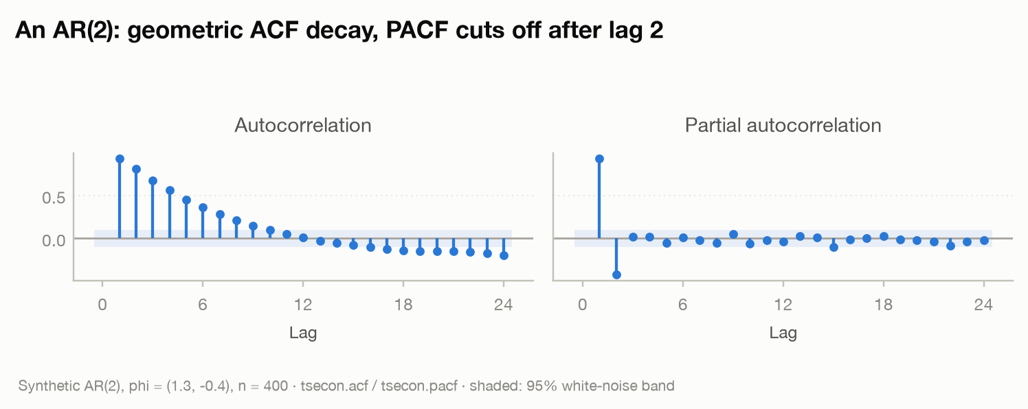
The synthetic series is an AR(2) with φ = (1.3, −0.4): the ACF decays smoothly (with a hint of oscillation), while the PACF shows exactly two spikes and then dies — read "fit an AR(2)" straight off the plot. Matches statsmodels at 1e-12.
2 · The stationarity workflow
Use case: before fitting anything, decide whether the series needs
differencing. Running ADF alone is a common mistake — ADF's null is a unit
root, KPSS's null is stationarity, and only together do they give a
confident answer. check_stationarity() runs both and classifies the
confirmatory quadrant.
rep = tsecon.check_stationarity(y)
rep["quadrant"]         # "Stationary" | "UnitRoot" | "Conflict" | "Inconclusive"
rep["recommendation"]   # "Proceed" | "Difference" | "Detrend"
rep["interpretation"]   # a plain-language explanation of the evidence
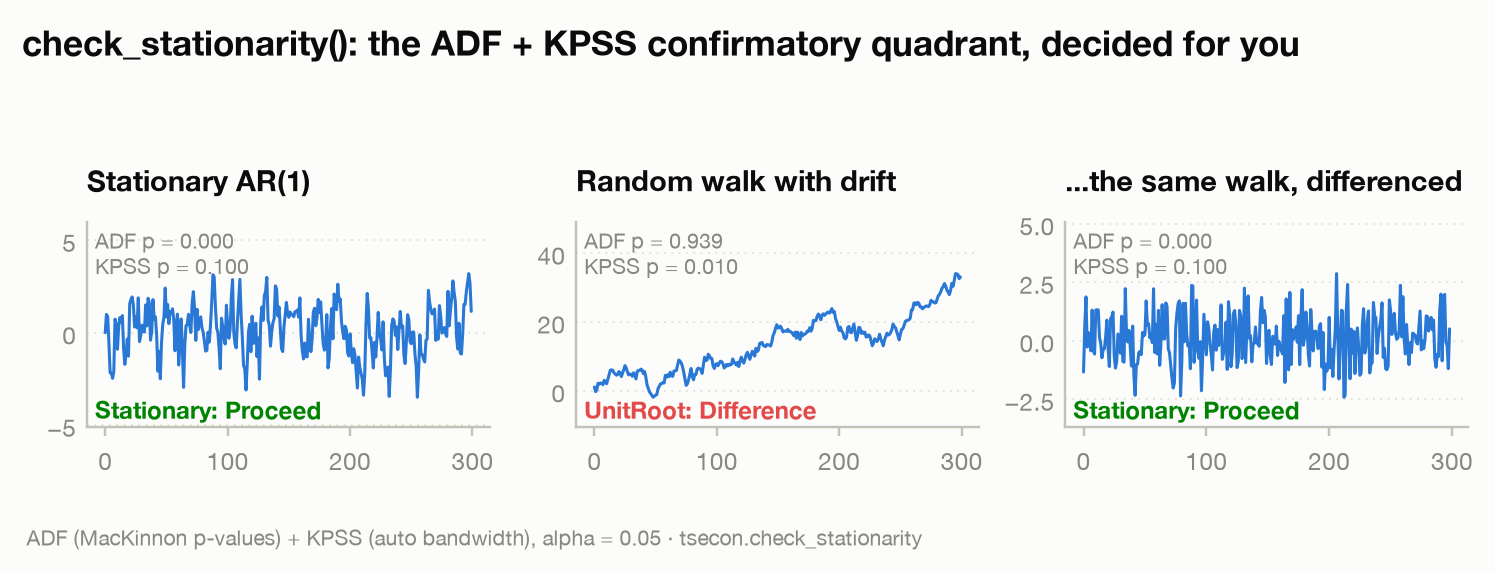
Left to right: a stationary AR(1) (both tests agree: proceed), a random walk
with drift (both tests agree: difference it), and the differenced walk
(proceed) — the workflow loop closes. The underlying tsecon.adf carries the
full MacKinnon p-value response surfaces; tsecon.kpss uses the
Hobijn-Franses-Ooms automatic bandwidth. Both match statsmodels at 1e-8.
3 · Robust standard errors (HAC / Newey-West)
Use case: any regression on time series data. With autocorrelated errors, textbook OLS standard errors are too small — you'll find "significant" effects that aren't there. HAC (heteroskedasticity- and autocorrelation-consistent) standard errors fix the variance estimate without changing the coefficients.
r = tsecon.ols(y, X, se_type="hac")          # Newey-West, automatic bandwidth
r = tsecon.ols(y, X, se_type="hac", maxlags=8)
r = tsecon.ols(y, X, se_type="hc1")          # heteroskedasticity-only
tsecon.long_run_variance(x, kernel="qs")     # the underlying LRV machinery
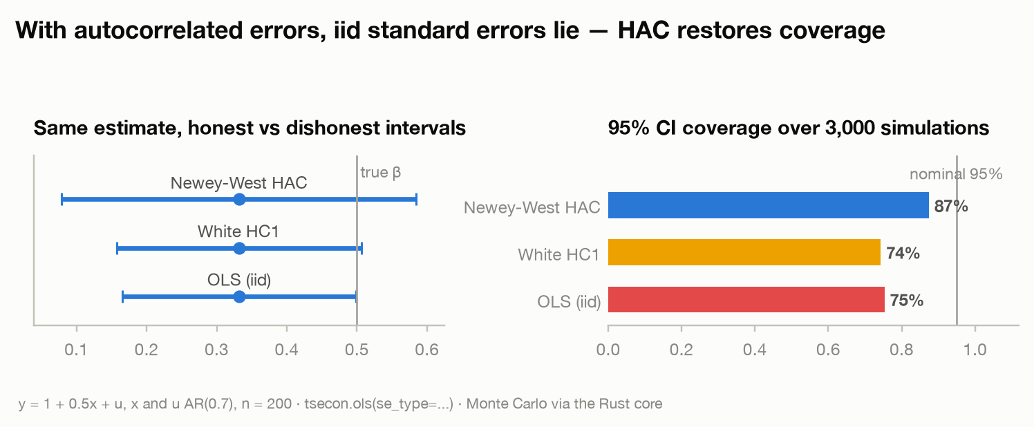
Left: one representative sample where the naive intervals only just graze
the true β while the wider HAC interval covers it comfortably. Right: the
same comparison run 3,000 times (9,000 regressions, seconds through the
Rust core): nominal 95% intervals cover only ~75% of the time under iid or
White standard errors; Newey-West restores most of the gap (the remainder is
the well-known small-sample HAC undercoverage — the roadmap's EWC fixed-b
inference, already implemented in the crate, is the modern answer).
HAC standard errors match statsmodels cov_type="HAC" at 1e-10 with
use_correction matched (the defaults differ: tsecon defaults the
finite-sample n/(n−k) correction on, statsmodels off — pass
use_correction=False to reproduce a default statsmodels call).
4 · Bootstrap for dependent data
Use case: inference when asymptotics are dubious — small samples, non-normal data, complicated statistics. The catch with time series: naive iid resampling destroys the dependence structure and gives you confidence intervals that are far too narrow. Block schemes resample contiguous chunks to preserve it.
opt = tsecon.optimal_block_length(y)                   # Politis-White (2004)
idx = tsecon.bootstrap_indices(n, scheme="stationary", # Politis-Romano
                               seed=b, p=1/opt["stationary"])
resampled = y[idx]
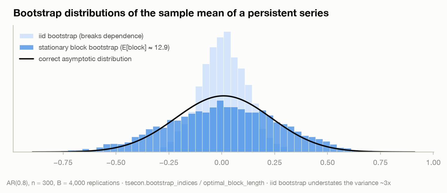
The bootstrap distribution of the sample mean of an AR(0.8) series, 4,000 replications: the iid bootstrap (light) is dramatically overconfident — about 3× too narrow — while the stationary block bootstrap (dark) with the automatically selected block length lands on the correct asymptotic distribution (black curve). Wild bootstrap weights (Rademacher, Mammen) are also available for regression settings. Same seed ⇒ bit-identical draws at any thread count.
5 · State-space models and the Kalman filter
Use case: extracting an unobserved signal from noisy measurements — trend extraction, missing-data interpolation, and the estimation engine under ARIMA, unobserved-components, and nowcasting models. This is the library's single most load-bearing component: exact diffuse initialization, missing data handled natively.
r = tsecon.local_level_smooth(y, sigma2_eps=4.8, sigma2_eta=0.5)
r["smoothed_state"]       # E[level_t | all data]  — NaNs bridged automatically
r["smoothed_state_var"]   # honest uncertainty, wider where data are missing
tsecon.ar_loglik(y, [0.6, -0.2], sigma2=1.4, intercept=1.5)  # exact MLE kernel
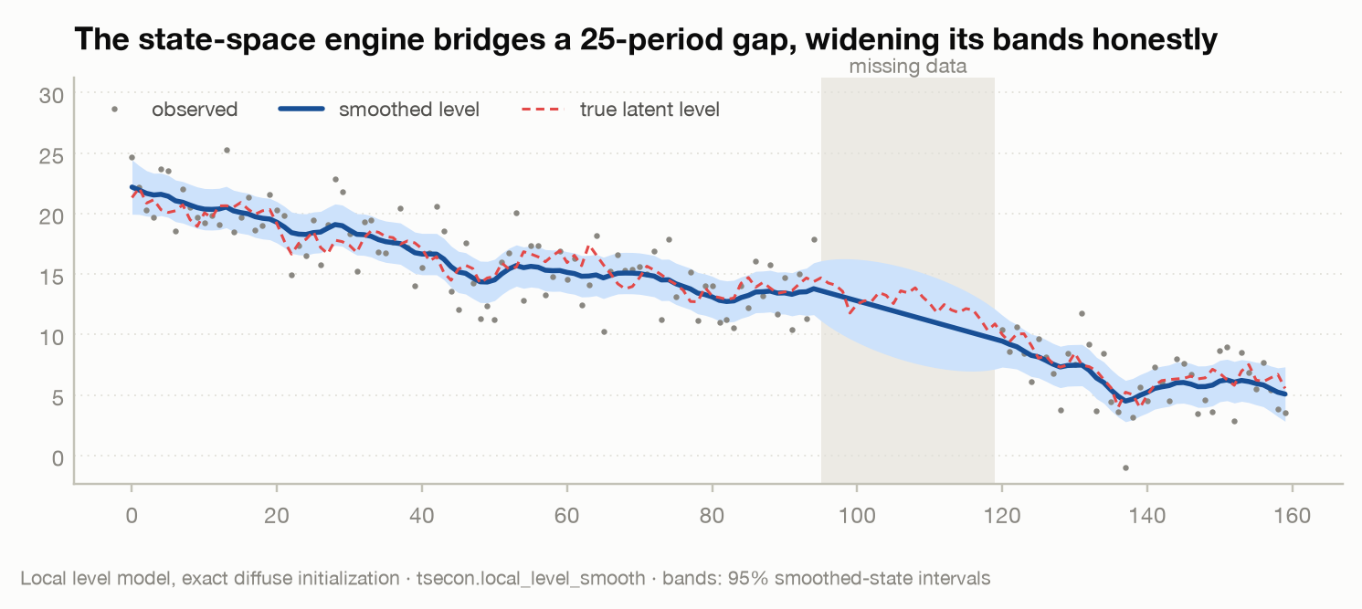
A local-level model with a 25-period gap in the observations: the smoother bridges the gap, the 95% band balloons exactly where information is missing, and the true latent path (dashed, never seen by the model inside the gap) stays within the band. Matches statsmodels' exact-diffuse results at ~1e-11.
6 · VAR: impulse responses and variance decomposition
Use case: the workhorse of empirical macro — how does a system of variables respond dynamically to a shock in one of them? Fit a VAR, identify shocks (Cholesky here; the full identification suite is Module 06), and read off impulse responses and variance decompositions.
r    = tsecon.var_fit(data, lags=2)                 # params, sigma_u, ICs, stability
irf  = tsecon.var_irf(data, lags=2, horizon=16)     # [h][response][shock]
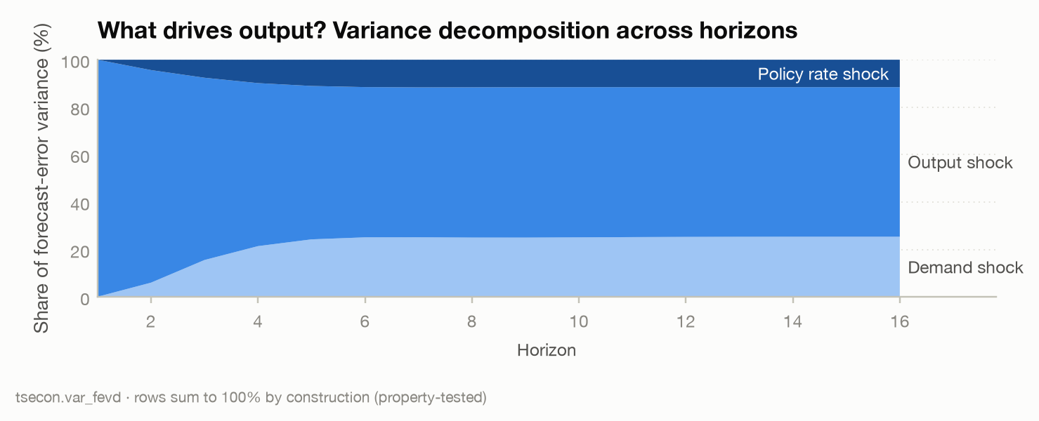
fevd = tsecon.var_fevd(data, lags=2, horizon=16)   # [h][variable][shock]
g    = tsecon.var_granger(data, caused=[0], causing=[1], lags=2)
fc   = tsecon.var_forecast(data, lags=2, steps=8)   # point + intervals
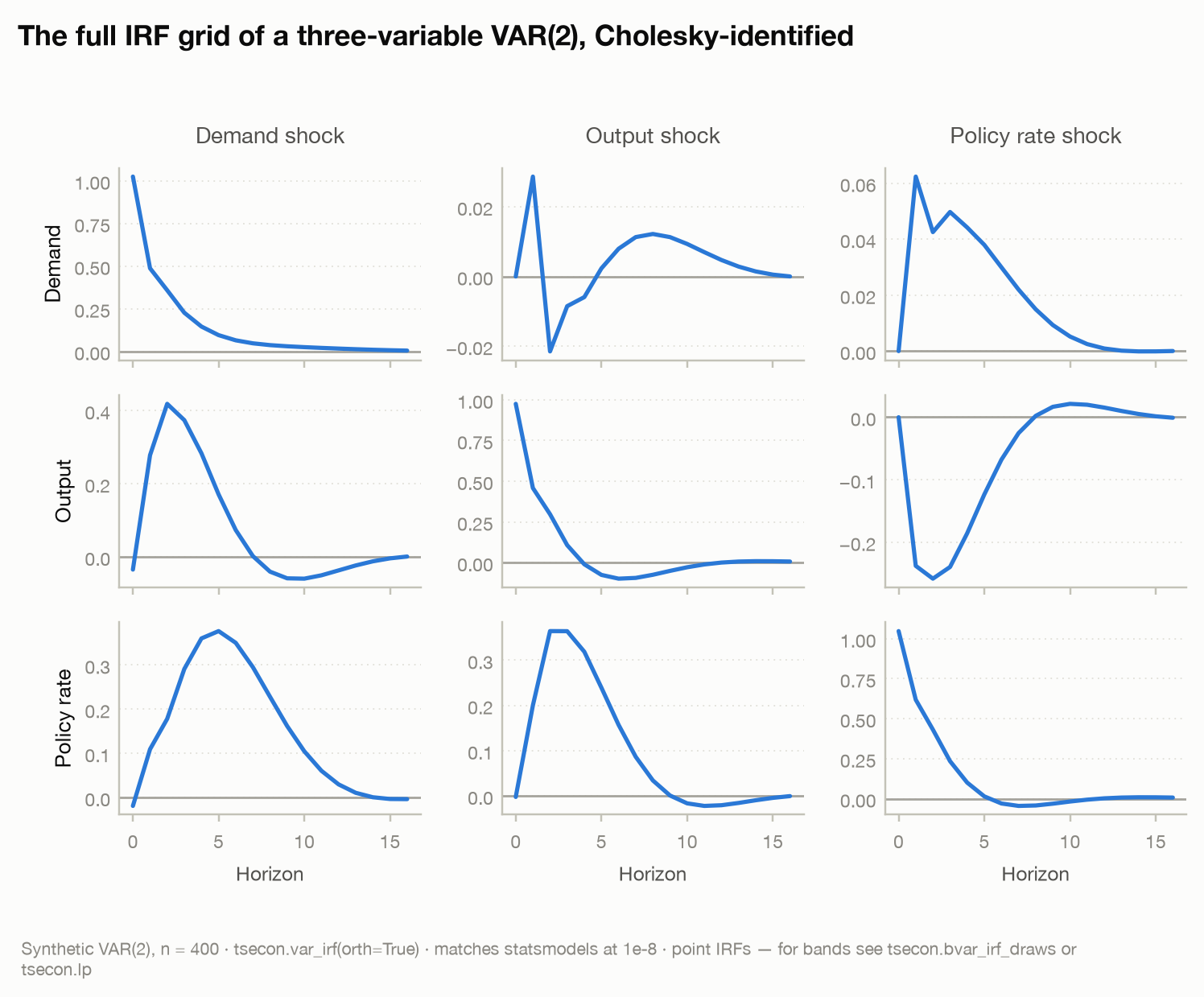
The synthetic system has a built-in causal story (demand moves first, output responds with a lag, the policy rate leans against both), and the estimated IRF grid recovers it — including the near-zero response of demand to output shocks that the recursive ordering implies. Every array matches statsmodels at 1e-8.
7 · Trend-cycle filters
Use case: separating the business cycle from the trend. This is a methodological minefield — Hamilton (2018) famously argued "why you should never use the HP filter" — so the library ships the alternatives side by side and makes their disagreement visible rather than hiding it.
hp  = tsecon.hp_filter(gdp, lamb=1600.0)       # + one_sided=True real-time variant
ham = tsecon.hamilton_filter(gdp, h=8, p=4)    # the modern alternative
bk  = tsecon.bk_filter(gdp, low=6, high=32, k=12)
cf  = tsecon.cf_filter(gdp, low=6, high=32)
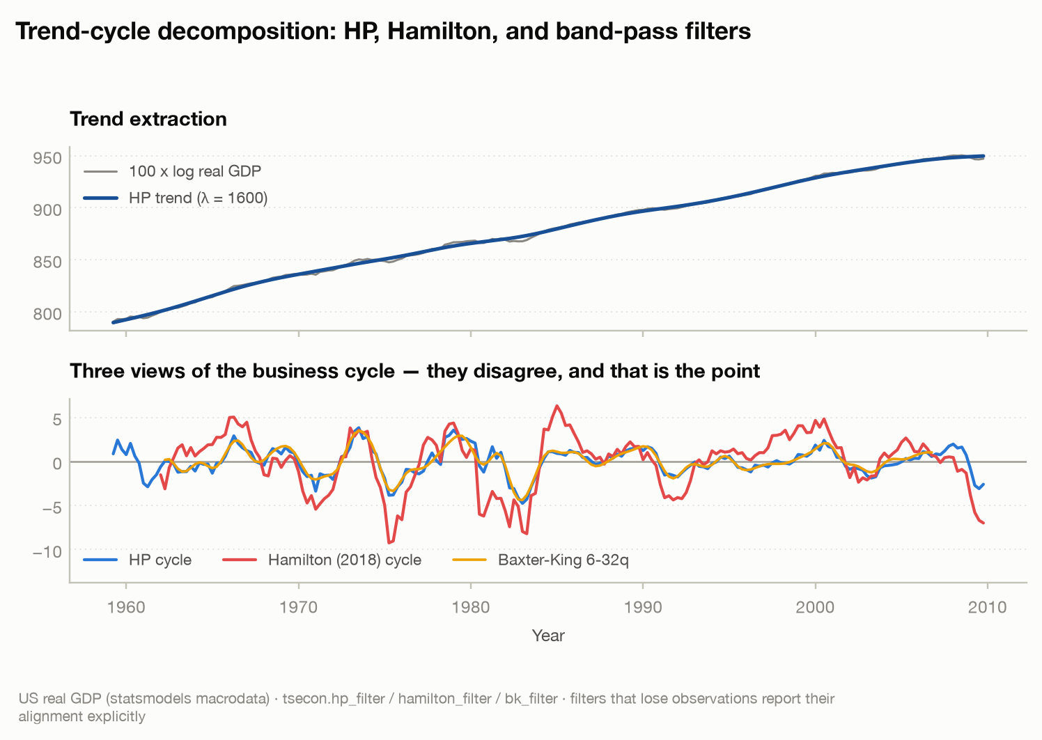
Real US GDP: the HP and Baxter-King cycles broadly agree; the Hamilton
filter reads recessions deeper and turns later — a genuine methodological
difference, not a bug. Filters that lose observations return explicit
alignment metadata (first_index) so nothing silently misaligns. HP runs
through an O(n) pentadiagonal solver, never a dense matrix.
8 · Forecast evaluation
Use case: the discipline layer. Never report a forecast without a benchmark and never claim superiority without a test. MASE scales errors by an in-sample naive forecast (1.0 = "no better than naive"); the Diebold-Mariano test asks whether an accuracy difference is statistically real, with the Harvey-Leybourne-Newbold small-sample correction.
fc  = tsecon.theta_forecast(y, steps=20, period=4)   # the M3-winning benchmark
acc = tsecon.accuracy(actual, fc, insample=train, period=4)  # rmse/mae/mase/...
dm  = tsecon.dm_test(e_benchmark, e_model, h=1, loss="squared")
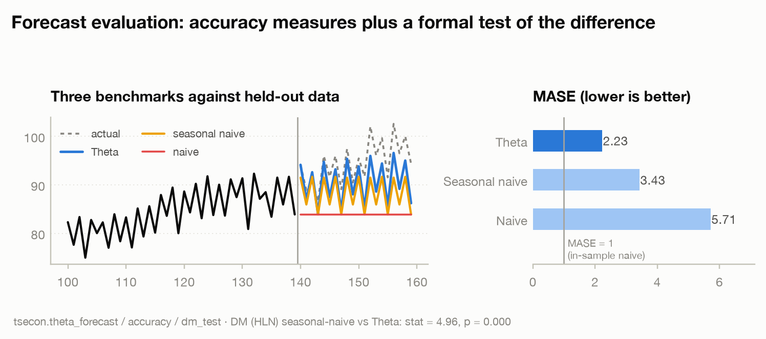
Theta beats the seasonal naive decisively here (MASE 2.23 vs 3.43, with the plain naive at 5.71; DM stat 4.96, p = 0.000) — and the plot shows why: it captures both the trend and the seasonal shape. The DM statistic matches the documented reference case at 1e-10.
9 · GARCH: volatility and risk
Use case: any application where the size of movements matters — risk management, option pricing, portfolio construction. Volatility clusters (calm and stormy periods alternate), which makes it forecastable even when returns themselves are not.
r = tsecon.garch_fit(returns, vol="garch", dist="normal", forecast_horizon=60)
r["params"], r["se_robust"]         # QMLE + Bollerslev-Wooldridge robust SEs
r["conditional_volatility"]         # the fitted sigma_t path
r["variance_forecast"]              # analytic multi-step, mean-reverting
# also: vol="gjr" (asymmetry), vol="egarch", dist="t" (fat tails)
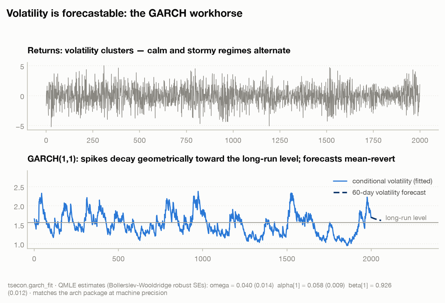
The fitted persistence (α + β ≈ 0.98) says volatility shocks take months to
die out — the long-run anchor and mean-reverting forecast fan follow
directly. Fixed-parameter likelihoods match Kevin Sheppard's arch package
at machine precision, and our optimizer's fits match or beat arch's optimum
on every golden case.
10 · Bayesian VAR: posterior impulse responses
Use case: VARs have many parameters and macro samples are short — the frequentist answer is noisy IRFs. The Bayesian answer is shrinkage: the Minnesota prior pulls coefficients toward a random-walk baseline, and the conjugate Normal-inverse-Wishart structure gives the entire posterior in closed form — no MCMC, no convergence worries, with the log marginal likelihood available to tune prior tightness on the evidence.
post = tsecon.bvar_fit(data, lags=2, lambda1=0.2)      # closed-form posterior
post["log_marginal_likelihood"]                         # evidence, for tuning
draws = tsecon.bvar_irf_draws(data, lags=2, horizon=12,
                              n_draws=800, seed=42)     # [draw][h][var][shock]
bands = np.quantile(draws, [0.05, 0.16, 0.5, 0.84, 0.95], axis=0)
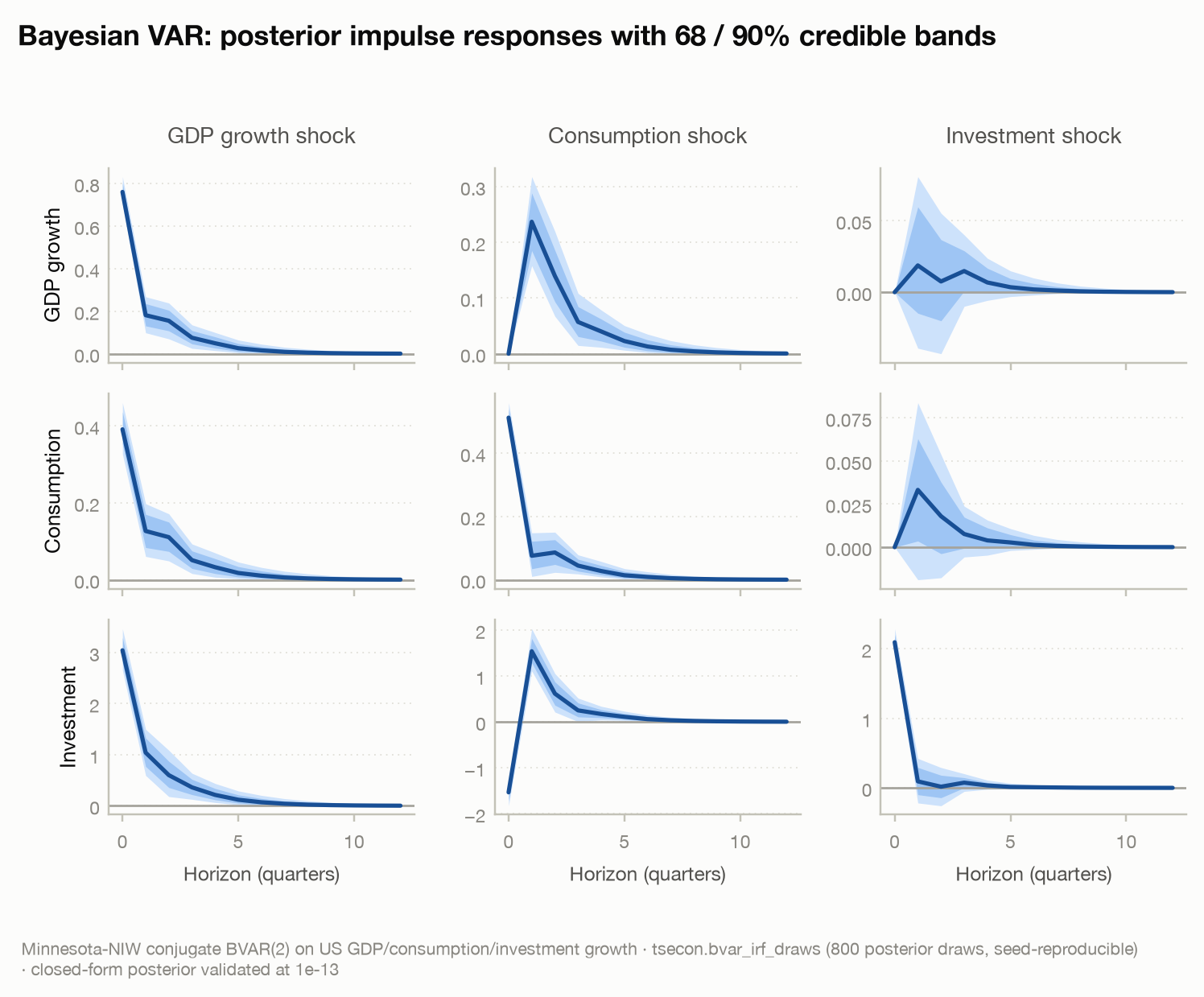
Real US data (GDP, consumption, investment growth): posterior medians with
nested 68/90% credible bands from 800 seed-reproducible posterior draws.
The analytic posterior is validated against the documented conjugate
updating equations at 1e-13; MCMC diagnostics (tsecon.mcmc_diagnostics:
ArviZ-exact R-hat and ESS) stand ready for the sampler-based models that
follow.
11 · ARIMA: fit, forecast, fan chart
Use case: the default univariate forecasting model. Difference to stationarity, capture short-run dynamics with AR and MA terms, forecast, and undifference — with uncertainty that compounds correctly across the integration.
r = tsecon.arima_fit(y, p=1, d=1, q=1, constant=True, forecast_steps=16)
r["params"], r["loglik"], r["aic"]      # exact MLE via the Kalman engine
r["forecast_mean"], r["forecast_se"]     # undifferenced, exact cumulative variance
tsecon.ljung_box(r["residuals"])         # adequacy check: residuals ~ white noise?
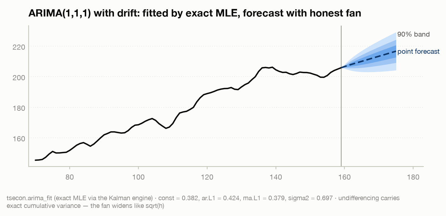
Fitted by exact maximum likelihood (Monahan-transformed L-BFGS with Hannan-Rissanen starting values), the fan widens like √h exactly as the random-walk-plus-dynamics theory requires. A validation note worth telling: on the Nile benchmark our optimizer found a better optimum than the one statsmodels' default fit had stored in our golden fixture — the fixture had pinned a non-converged artifact, which independent cross-checking confirmed. Validation-first development cuts both ways.
Advanced
The numbered sections showed the methods one at a time. This wing composes them: four figures from the sophisticated end of applied practice, each built entirely from the primitives above. All regenerate with one command:
Local projections (Jordà 2005), from primitives
Use case: the modern default for estimating impulse responses without
committing to a full VAR's dynamics — run one regression per horizon of
y[t+h] on the shock (plus lag controls) and read the IRF straight off the
shock coefficients. The h-step regression error is MA(h) by construction, so
HAC standard errors are not optional — which is exactly what tsecon.ols
provides.
for h in range(13):
    t = np.arange(4, n - h)
    X = np.column_stack([np.ones(len(t)), shock[t]]
                        + [y[t - lag] for lag in range(1, 5)])
    r = tsecon.ols(y[t + h], X, se_type="hac", maxlags=h + 1)
    irf[h], se[h] = r["params"][1], r["bse"][1]   # band: irf ± 1.645·se
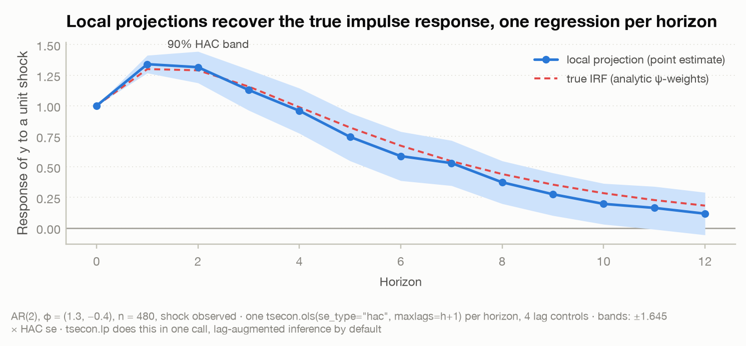
The test bed is an AR(2) whose true impulse response is computable
analytically (the ψ-weights, dashed red), and the local projection tracks it
inside its 90% HAC bands at every horizon — including the hump at h = 1 and
the long geometric tail. This is Jordà (2005) built from tsecon primitives
by hand; the shipped tsecon.lp (Module 07)
packages the same estimator with lag-augmented inference as its default —
see the structural wing below.
News impact curves: is volatility asymmetric?
Use case: in equity markets, bad news famously raises tomorrow's
volatility more than good news of the same size. The news impact curve
(Engle-Ng 1993) makes the question visual: plot the fitted σ²(ε) against the
shock ε, holding the lagged variance at its unconditional level. GARCH is a
symmetric parabola by construction; GJR adds a gamma term that kinks the
curve at zero.
gj = tsecon.garch_fit(ret, vol="gjr", mean="zero")     # and vol="garch"
om, al, ga, be = gj["params"]
s2 = om / (1 - al - ga / 2 - be)                       # unconditional variance
nic = om + (al + ga * (eps < 0)) * eps**2 + be * s2    # the curve
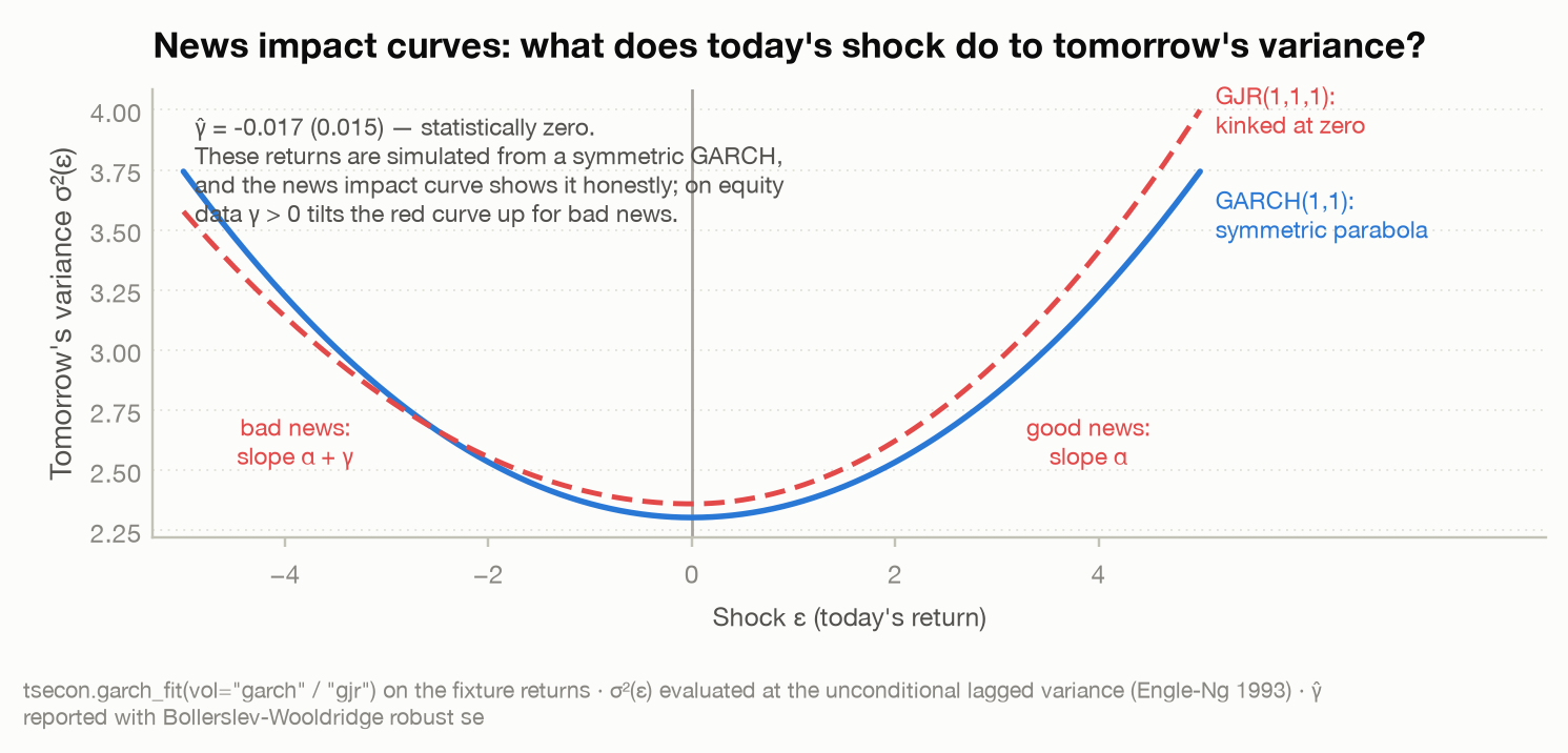
An honest negative result, on purpose: the fixture returns are simulated from a symmetric GARCH, and the fitted GJR says so — γ̂ = −0.017 with a robust standard error of 0.015, statistically zero, so the two curves nearly coincide. That is the diagnostic working as designed: fit GJR, draw the curve, and let the kink (or its absence) tell you whether the leverage effect is in your data. On real equity returns γ̂ > 0 tilts the curve up steeply on the bad-news side.
The volatility term structure
Use case: risk over horizons — option pricing, margin setting, VaR at one day versus six months. A GARCH fit implies a whole term structure of expected volatility: from any starting state, forecasts decay toward the long-run anchor at rate α + β per period, and the fitted persistence tells you how slowly.
r = tsecon.garch_fit(ret, vol="garch", mean="zero", forecast_horizon=120)
term = np.sqrt(r["variance_forecast"])        # from the end-of-sample state
om, al, be = r["params"]
lr = om / (1 - al - be)                       # the long-run anchor
what_if = lr + (al + be) ** (h - 1) * (3 * lr - lr)   # closed-form, any state
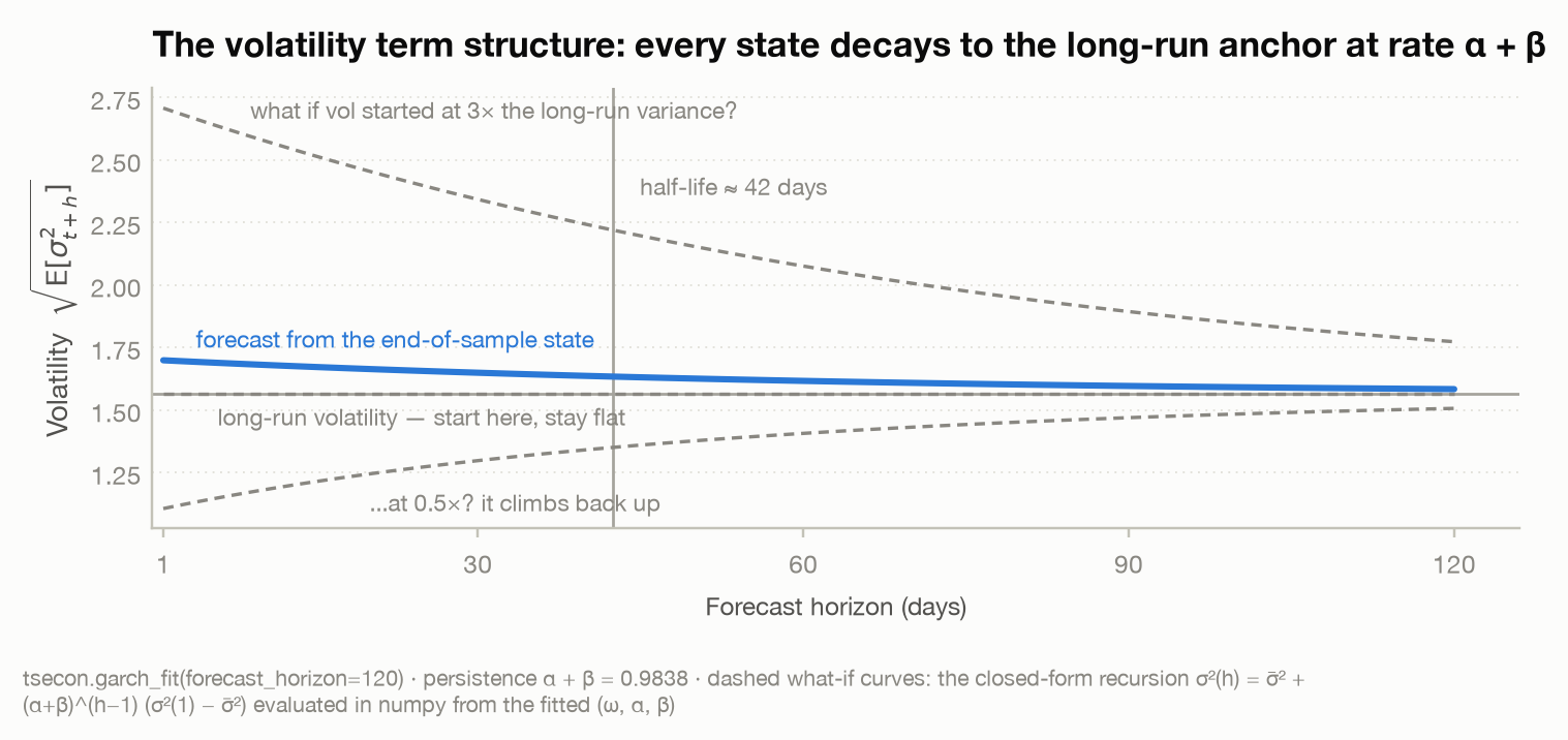
The solid blue curve is the library's own variance_forecast, launched from
the actual end-of-sample state. The API forecasts only from that state, so
the dashed what-if curves (starting at 0.5×, 1×, and 3× the long-run
variance) are the same closed-form recursion evaluated in numpy from the
fitted (ω, α, β) — labelled as such. With persistence α + β = 0.9838 the
half-life of a volatility shock is about 42 trading days: spikes are not
noise, they are two-month weather systems.
BVAR prior tightness in one picture
Use case: the Minnesota prior's λ₁ is the shrinkage knob — how hard the data must argue against the random-walk baseline. Set it by eye and you're guessing; the conjugate NIW posterior gives the log marginal likelihood in closed form, so the evidence can pick it. This figure shows what the choice does where it matters: the impulse response and its uncertainty.
for lam in [0.05, 0.2, 1.0]:
    draws = np.array(tsecon.bvar_irf_draws(data, lags=2, horizon=12,
                                           n_draws=500, seed=42, lambda1=lam))
    gg = draws[:, :, 0, 0]                    # GDP response to a GDP shock
    lo, med, hi = np.quantile(gg, [0.05, 0.5, 0.95], axis=0)   # 90% band
    lml = tsecon.bvar_fit(data, lags=2, lambda1=lam)["log_marginal_likelihood"]
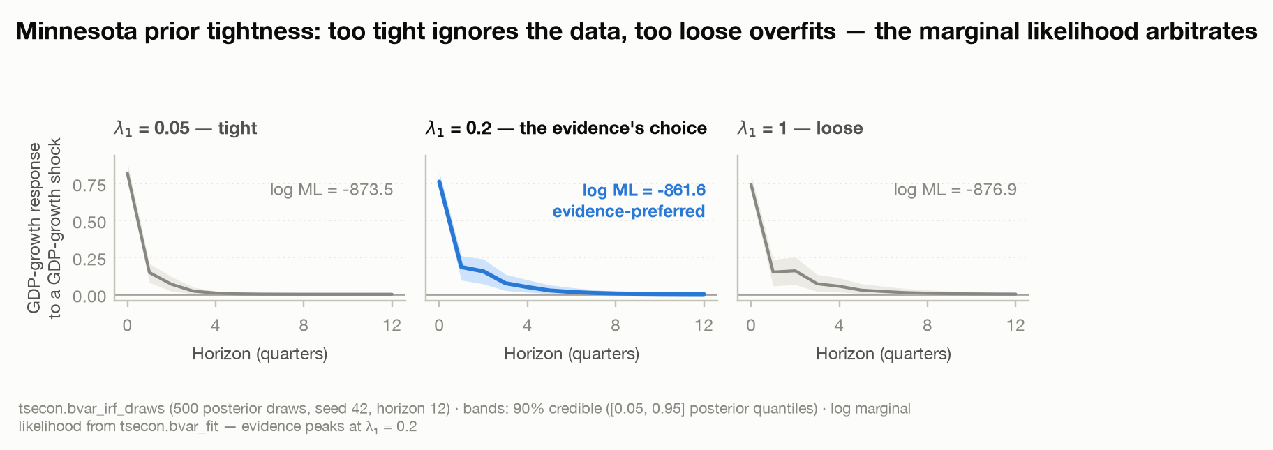
Too tight (λ₁ = 0.05) squeezes the response toward the prior and understates uncertainty; too loose (λ₁ = 1.0) is essentially OLS with wide, wobbly bands. The log marginal likelihood arbitrates: −873.5, −861.6, −876.9 — the evidence decisively prefers the middle setting, drawn in house blue. Same seed, same 500 draws per panel, so the differences you see are the prior, not Monte Carlo noise.
Structural & shrinkage
Three capabilities from the identification-and-regularization frontier — set-identified structural inference, honest local-projection bands, and penalized selection. Each figure is a real computation through the Rust core, and they regenerate with one command:
Sign-restricted SVAR: the identified set
Use case: recursive (Cholesky) identification forces a variable ordering you may not believe. Sign restrictions ask for less — only the signs of a few impact responses, the kind of thing theory actually delivers ("a demand shock raises output, consumption, and investment on impact") — and return every impulse response consistent with them. The answer is not a point: it is an interval at each horizon, the identified set.
restr = [(0, 0, 0, "+"), (1, 0, 0, "+"), (2, 0, 0, "+")]  # (var, shock, horizon, sign)
r = tsecon.sign_restricted_svar(data, restrictions=restr, horizon=12, n_draws=800)
r["set_min"], r["set_max"]     # identified-set envelope       [h][var][shock]
r["quantiles"]                 # posterior 5/16/50/84/95 within the set
r["diagnostics"]               # rotations tried, acceptance rate
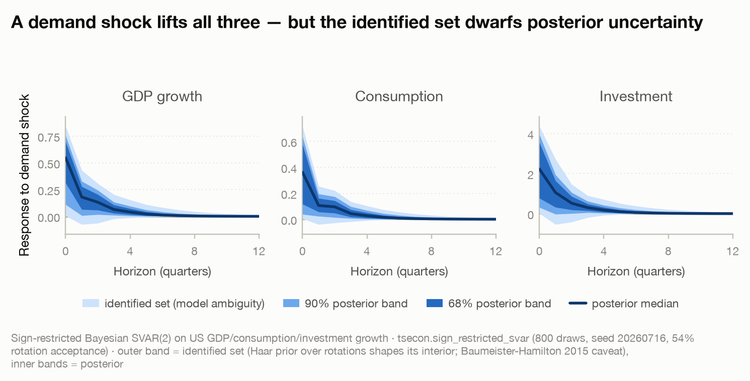
A demand shock lifts GDP growth, consumption, and investment on impact by
construction, then each decays. The figure keeps two very different kinds of
uncertainty visually separate: the lightest band is the identified set —
the range of responses the restrictions alone cannot rule out (model
ambiguity), and it is wide; the nested 68/90% bands inside it are posterior
(sampling) uncertainty given a rotation, and they are much narrower. The
Baumeister-Hamilton (2015) caveat is why the outer envelope, not the median,
is the honest object: the uniform (Haar) prior over rotations is not flat over
impulse responses, so it shapes the interior of the set even where the data
are silent. About 54% of candidate rotations satisfy the restrictions here,
reported in diagnostics.
Local projections with honest bands
Use case: the modern default for impulse responses (Jordà 2005) — one
regression of y[t+h] on the shock per horizon, with no VAR dynamics to
commit to. The subtlety is inference: the h-step error is serially correlated,
and the naive HAC band is known to under-cover at longer horizons. Montiel
Olea and Plagborg-Møller (2021) show that a lag-augmented projection
restores valid, uniform coverage with a one-line fix — and it is tsecon.lp's
default.
la = tsecon.lp(y, shock, horizons=16)                 # se="lag_augmented" (the default)
hc = tsecon.lp(y, shock, horizons=16, se="hac")       # the older HAC alternative
lo, hi = la["irf"] - 1.6449 * la["se"], la["irf"] + 1.6449 * la["se"]   # 90% band
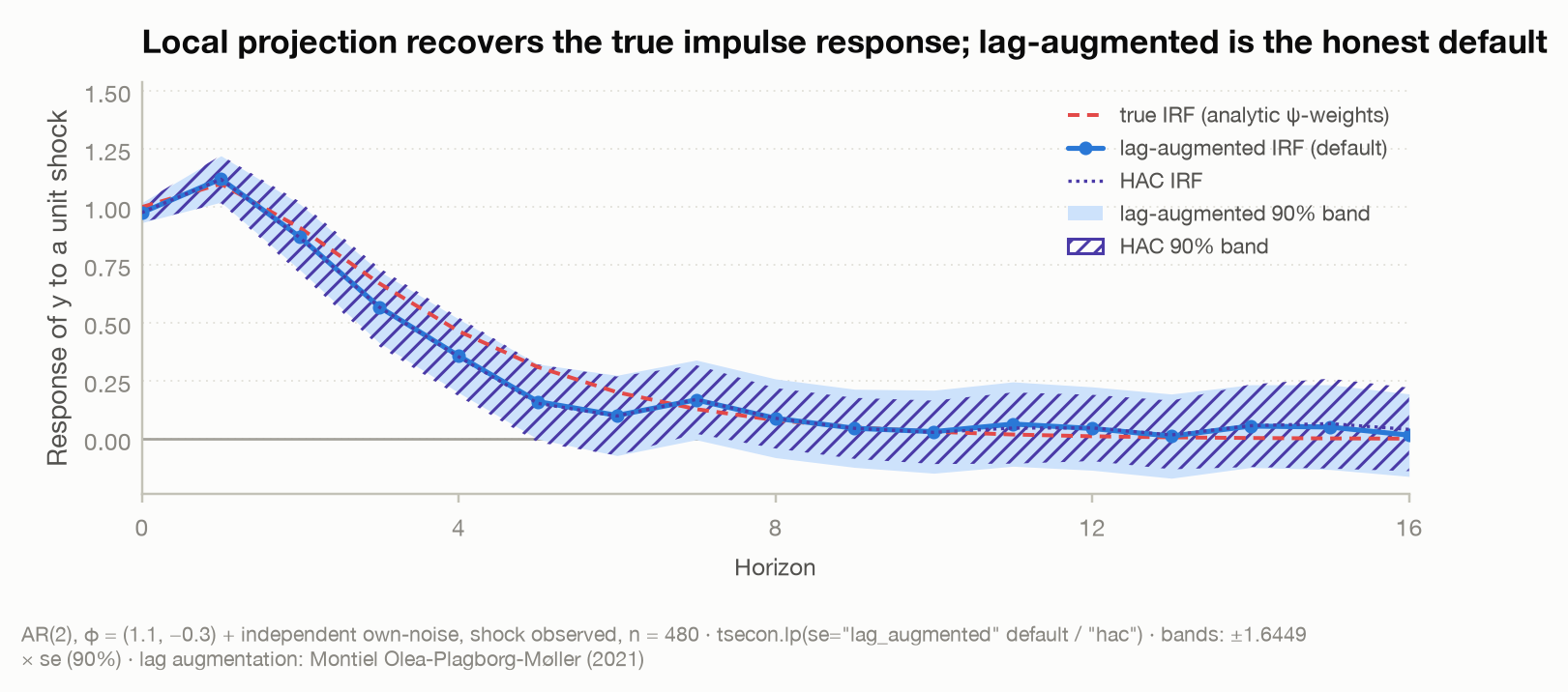
The test bed is an AR(2) driven by an observed shock, whose true impulse
response is the analytic ψ-weights (dashed red) — so the recovery is checkable
directly. Both the lag-augmented default and the HAC projection track the
truth at every horizon, and their point estimates all but coincide. What
differs is the bands: drawn with distinct fills, the two schemes disagree
about width, and lag augmentation is the one carrying the coverage guarantee.
Use it by default; reach for se="hac" only to reproduce older results.
tsecon.lp_iv extends the same machinery to instrumented shocks with a
first-stage F diagnostic.
The lasso path: shrinkage as selection
Use case: many candidate predictors, most of them noise — the setting where OLS overfits and you want the model itself to choose. The lasso's L1 penalty does double duty: it shrinks coefficients and sets most of them exactly to zero, so fitting and variable selection happen in one step. Sweeping the penalty α traces the classic coefficient path.
alphas = np.logspace(-2, 0.5, 60)                     # weak (small) → strong (large)
paths = np.array([tsecon.lasso(Xs, y, alpha=a)["coef"] for a in alphas])
# same core, other objectives:
tsecon.ridge(Xs, y, alpha)                            # shrink, never select
tsecon.elastic_net(Xs, y, alpha, l1_ratio=0.5)        # the in-between
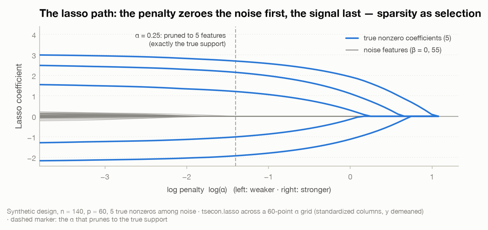
A synthetic design hides five true nonzero coefficients among 55 pure-noise
features. Read right to left as the penalty weakens: the five signal
coefficients (house blue) emerge in order of strength, while the noise
features (muted) stay pinned near zero until α is very small. The dashed
marker is the penalty that prunes the model to exactly five features — and
here those five are exactly the true support: sparsity delivering correct
selection, not merely a smaller model. Ridge (tsecon.ridge) and the elastic
net (tsecon.elastic_net) share the same coordinate-descent core for the
shrink-don't-select and in-between cases.
Depth methods
Score-driven volatility: the robust Student-t GAS
Use case: volatility estimation when returns have fat tails and the occasional jump — the setting where a Gaussian GARCH-style filter over-reacts to a single large shock and reports spurious persistence. A GAS (generalized autoregressive score) model drives the variance by the score of the observation density; with a Student-t density that score down-weights outliers automatically.
r = returns                                   # a return series with jumps
g  = tsecon.gas_volatility(r, density="gaussian")
st = tsecon.gas_volatility(r, density="student_t")   # estimates the dof nu
vol_gaussian = np.sqrt(g["variance"])
vol_student  = np.sqrt(st["variance"])        # far calmer at the jumps
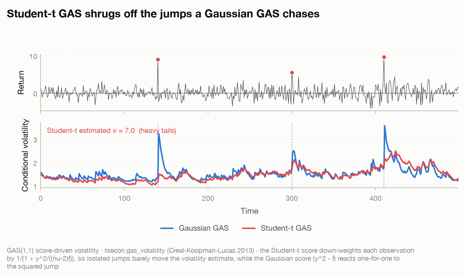
The return series (top) carries three isolated jumps (red). At each one
(dashed lines, bottom) the Gaussian GAS volatility (blue) spikes hard,
because its score y² − f reacts one-for-one to the squared shock; the
Student-t GAS (red) barely moves, because its score multiplies that shock by
1/(1 + y²/((ν−2)f)) — a soft-thresholding weight that treats a jump as a
tail draw, not a change in the underlying volatility. The estimated ν ≈ 7
confirms the heavy tails the model exploits.
Connectedness: who spills over to whom
Use case: measuring how shocks propagate across a system of markets or sectors — which are net transmitters of volatility and which are receivers. The Diebold-Yilmaz framework reads this straight off a VAR's generalized forecast-error-variance decomposition.
res = tsecon.connectedness(data, lags=1, horizon=10)   # data is T × k
res["total"]        # system-wide spillover index (%)
res["net"]          # per-variable net = to-others − from-others
res["gfevd"]        # the full directional spillover table (rows sum to 1)
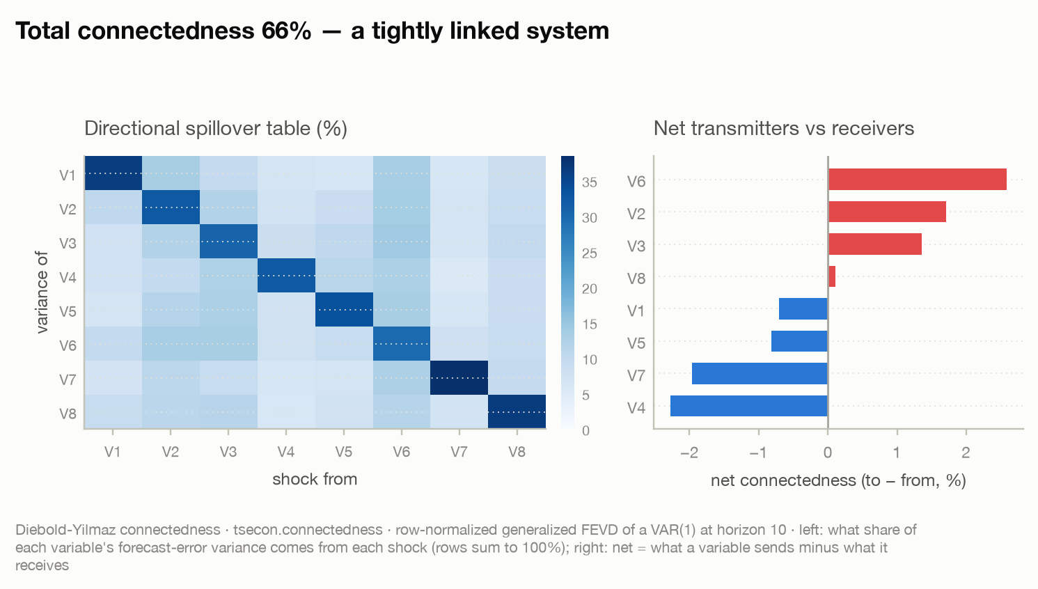
At a total connectedness of 66%, two-thirds of the system's forecast-error
variance is cross-variable, not own. The heatmap (left) is the directional
spillover table — row i, column j is the share of variable i's variance
driven by shocks to j; the strong off-diagonal is the connectedness. The
bars (right) rank each variable's net position: red variables transmit more
than they receive, blue ones the reverse.
FAVAR: one policy shock, many responses
Use case: you want the response of hundreds of series to a single identified shock without estimating a hundred-variable VAR. A factor-augmented VAR compresses the information set to a few factors, identifies the shock in that small system, and maps the responses back onto every series through the loadings.
res = tsecon.favar(panel, policy, n_factors=2, lags=2, horizon=24)
res["irf_policy"]   # the policy variable's own response
res["irf_panel"]    # every information-panel series' response (N × horizon+1)
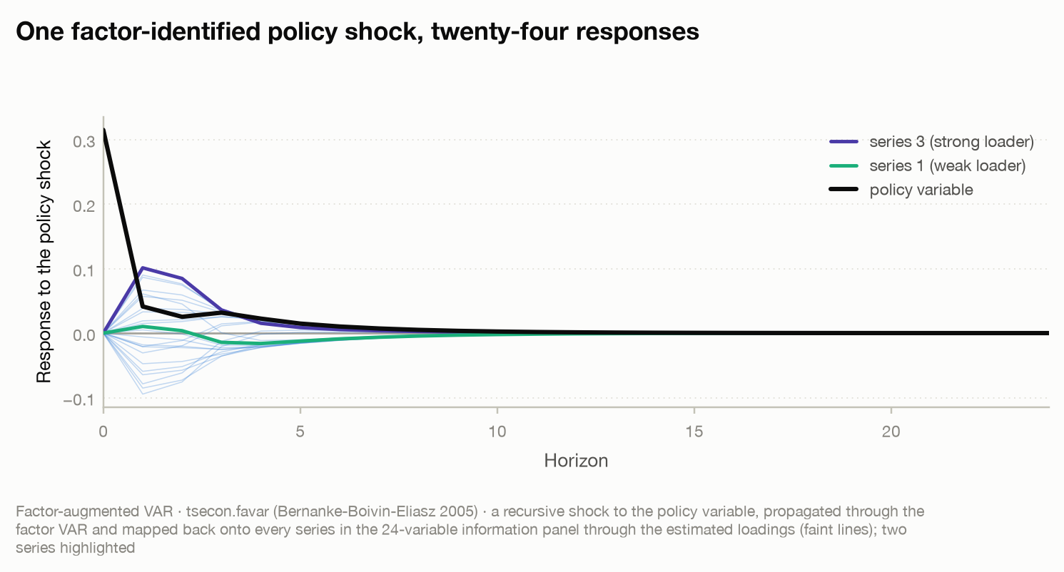
A recursive shock to the policy variable (bold) propagates through the factor VAR and, via the estimated loadings, onto all 24 series in the information panel (faint). Two are highlighted: a strong factor loader that moves visibly and a weak one that barely responds — the loadings decide who feels the shock.
The term structure in three numbers
Use case: summarizing an entire yield curve — dozens of maturities — with three interpretable factors (level, slope, curvature), and tracking how they move over time. The dynamic Nelson-Siegel model is the workhorse.
res = tsecon.dynamic_ns(panel, maturities, decay=0.0609)   # panel is T × n_maturities
res["level"], res["slope"], res["curvature"]               # the factor series
fit = tsecon.nelson_siegel(maturities, curve, decay=0.0609)  # one date's curve
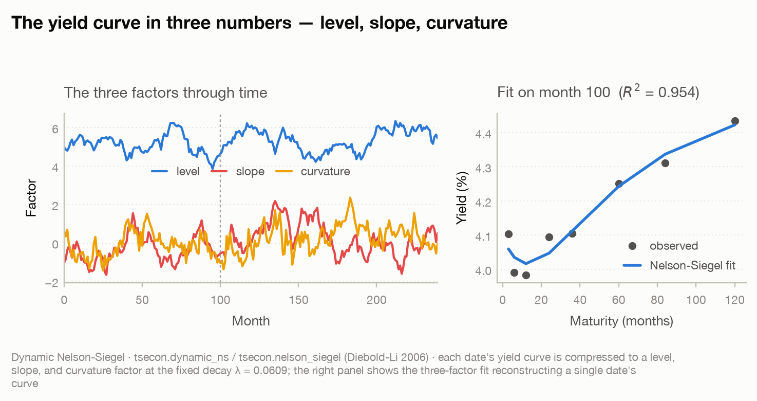
Each month's curve collapses to three numbers (left). The right panel shows the three-factor fit reconstructing a single date's curve to an \(R^2\) of 0.95 — a whole cross-section of yields captured by level, slope, and curvature.
Realized volatility: separating jumps from diffusion
Use case: with intraday data you can measure yesterday's volatility almost exactly — and split it into a smooth (diffusive) part and discrete jumps. Bipower variation is robust to jumps, so realized-variance-minus-bipower isolates the jump contribution, and the BNS ratio test says which days jumped.
m = tsecon.realized_measures(intraday_returns)   # one day of returns
m["rv"], m["bipower"], m["jump"]                 # total, continuous, jump
tsecon.bns_jump_test(intraday_returns)["ratio"]  # > 1.96 ≈ a 5% jump day
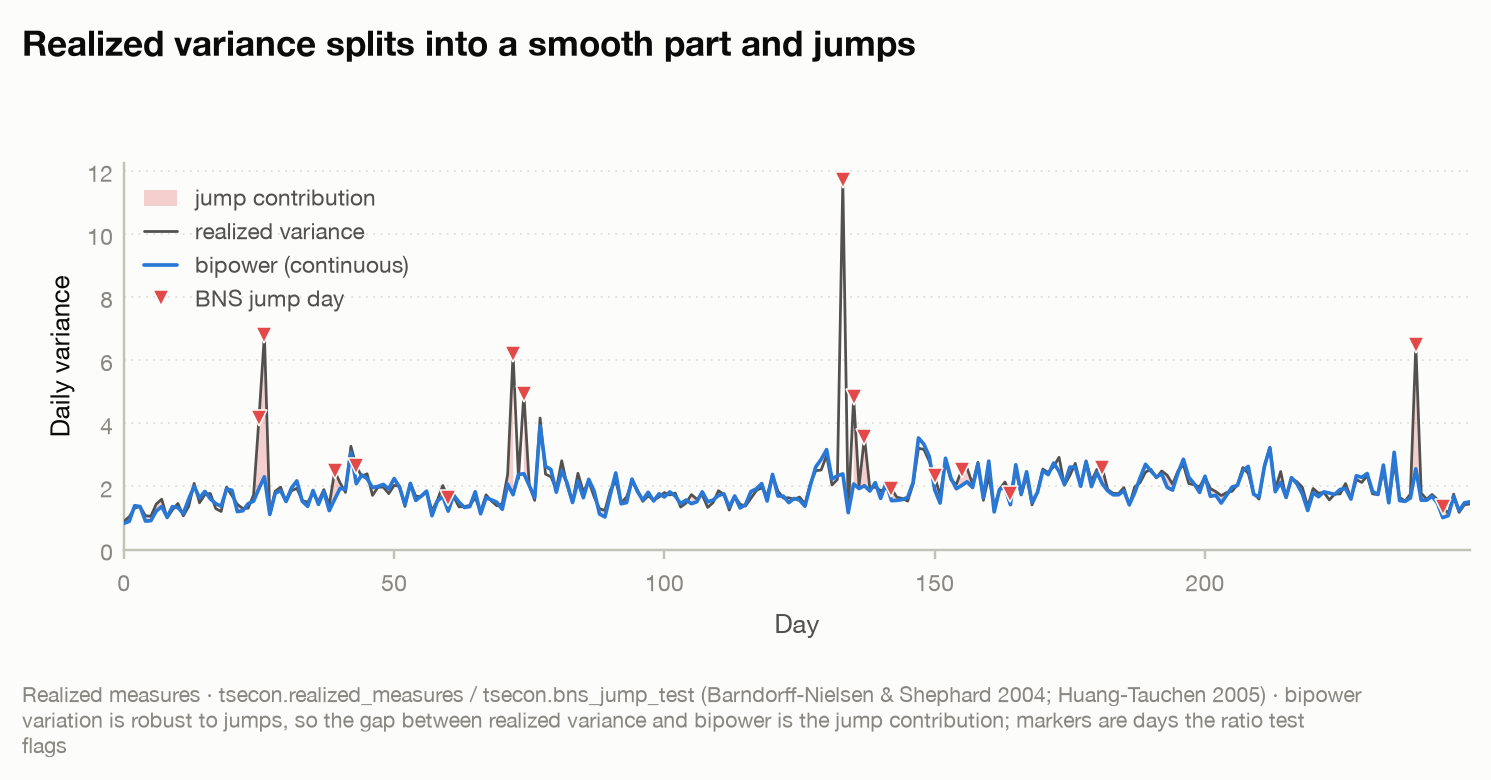
Realized variance (thin) sits at or above the jump-robust bipower variation (blue); the shaded gap is the jump contribution, and the markers are the days the BNS ratio test flags as jumps — the big spikes are discrete jumps, not a change in the underlying diffusion.
Mean group vs CCE: the common-factor bias, and its cure
Use case: a panel whose units have genuinely different slopes, contaminated by an unobserved common factor (a global cycle, a common shock). Plain mean-group averaging is biased; the common-correlated-effects estimator purges the factor by augmenting each unit with cross-section averages.
mg  = tsecon.panel_mean_group(ys, xs, method="mg")    # Pesaran-Smith 1995
cce = tsecon.panel_mean_group(ys, xs, method="cce")   # Pesaran 2006, factor-robust
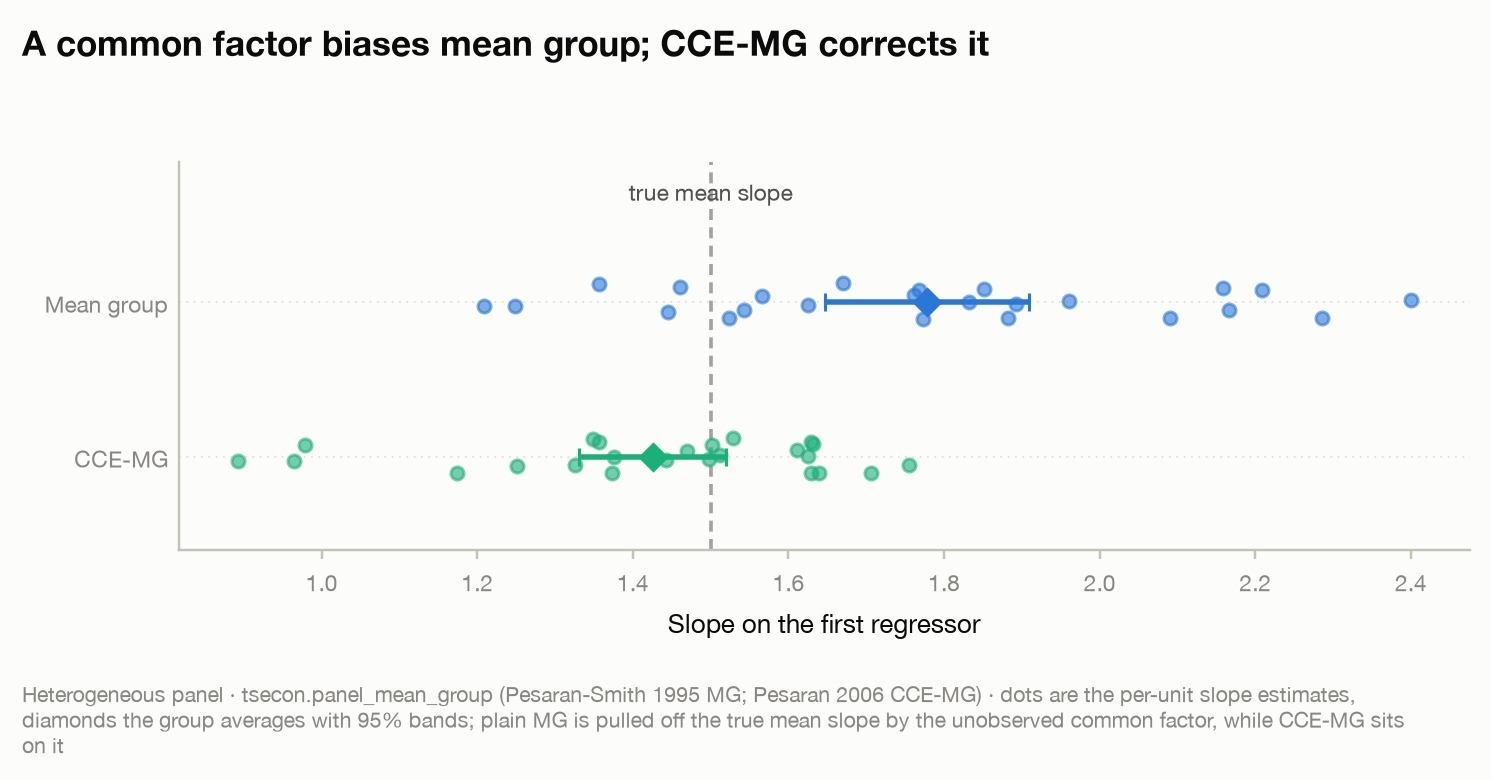
The dots are the per-unit slope estimates, the diamonds the group averages with 95% bands. Plain mean group (top) is pulled well to the right of the true mean slope by the common factor; CCE-MG (bottom) sits right on it — the correction the common-correlated-effects augmentation buys.
Roadmap extensions
The roadmap-E methods — recession probability, survey expectations, long memory, the CUSUM stability test, predictive regressions / IVX, the arbitrage-free Nelson-Siegel adjustment, and the linear rational-expectations (DSGE-lite) saddle path. All seven figures are generated by showcase_extensions.py:
Recession probability from a leading spread
Use case: turn a leading indicator — classically the term spread — into a
calibrated probability of recession. A probit (or the Kauppi-Saikkonen dynamic
probit) maps the spread to P(recession), the quantitative version of the
"inverted yield curve" warning.
X = np.column_stack([np.ones(n), spread])
fit = tsecon.recession_probit(y, X, link="probit")   # y is the 0/1 indicator
fit["probabilities"]     # fitted P(recession); also params, pseudo_r2, ...
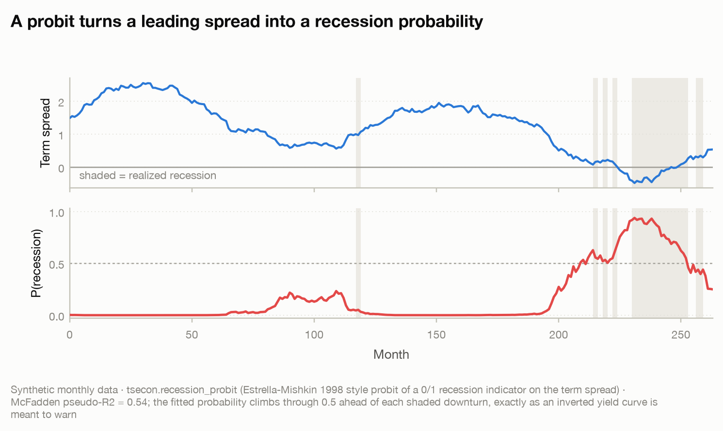
The spread (top) falls ahead of each shaded downturn; the fitted probability (bottom) climbs through 0.5 just before it, exactly as a leading indicator should. See the recession model card.
Survey expectations: rigidity and disagreement
Use case: test whether professional forecasts are fully rational and measure how much forecasters disagree. The Coibion-Gorodnichenko regression of the mean forecast error on the mean revision has slope zero under full-information rational expectations; a positive slope is the signature of information rigidity.
cg = tsecon.cg_regression(errors, revisions)   # HAC-robust; slope, implied_rigidity
dis = tsecon.forecast_disagreement(panel)      # per-period std, IQR, quantiles
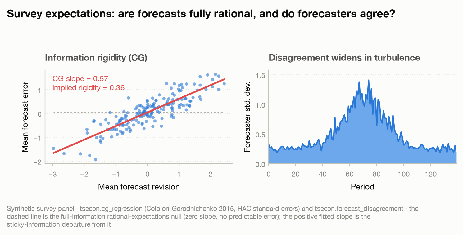
Left: the CG regression — the dashed line is the rational-expectations null (zero slope), the positive fit its sticky-information departure. Right: cross-sectional disagreement widening through a turbulent stretch. See the survey expectations card.
Long memory: a hyperbolic ACF and the filter that removes it
Use case: some series (realized volatility, inflation, trading volume) decay
too slowly for an ARMA but are not unit-root either — they have long memory,
0 < d < 0.5. Estimate d, then fractionally difference to whiten.
d_hat = tsecon.long_memory_d(x, method="local_whittle")["d"]   # Robinson 1995
x_white = tsecon.frac_diff(x, d_hat)                            # (1 - L)^d
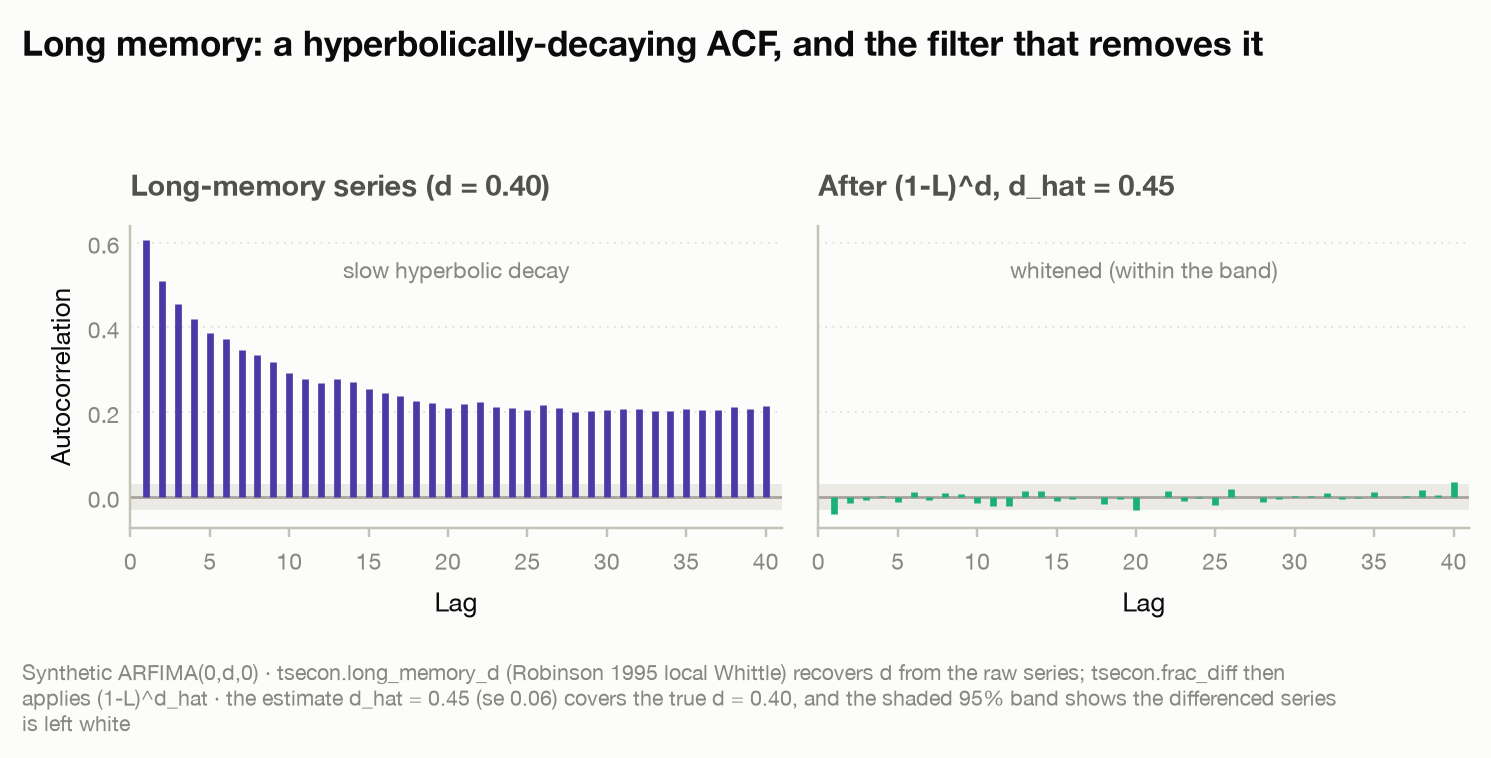
Left: the raw series' ACF decays hyperbolically — still 0.2 at lag 40. Right:
after (1 − L)^d̂ the autocorrelation sits inside the 95% band; the estimate
covers the true d = 0.40. See the
long-memory card.
CUSUM: parameter stability over the sample
Use case: did the regression relationship hold constant, or did the coefficients drift/break somewhere you did not pre-specify? The Brown-Durbin-Evans CUSUM of recursive residuals is a random walk near zero under stable coefficients and walks out of its 5% band when they shift.
cs = tsecon.cusum_test(y, X)          # path, bound_upper, bound_lower, sigma
breach = np.any(cs["path"] > cs["bound_upper"]) or np.any(cs["path"] < cs["bound_lower"])
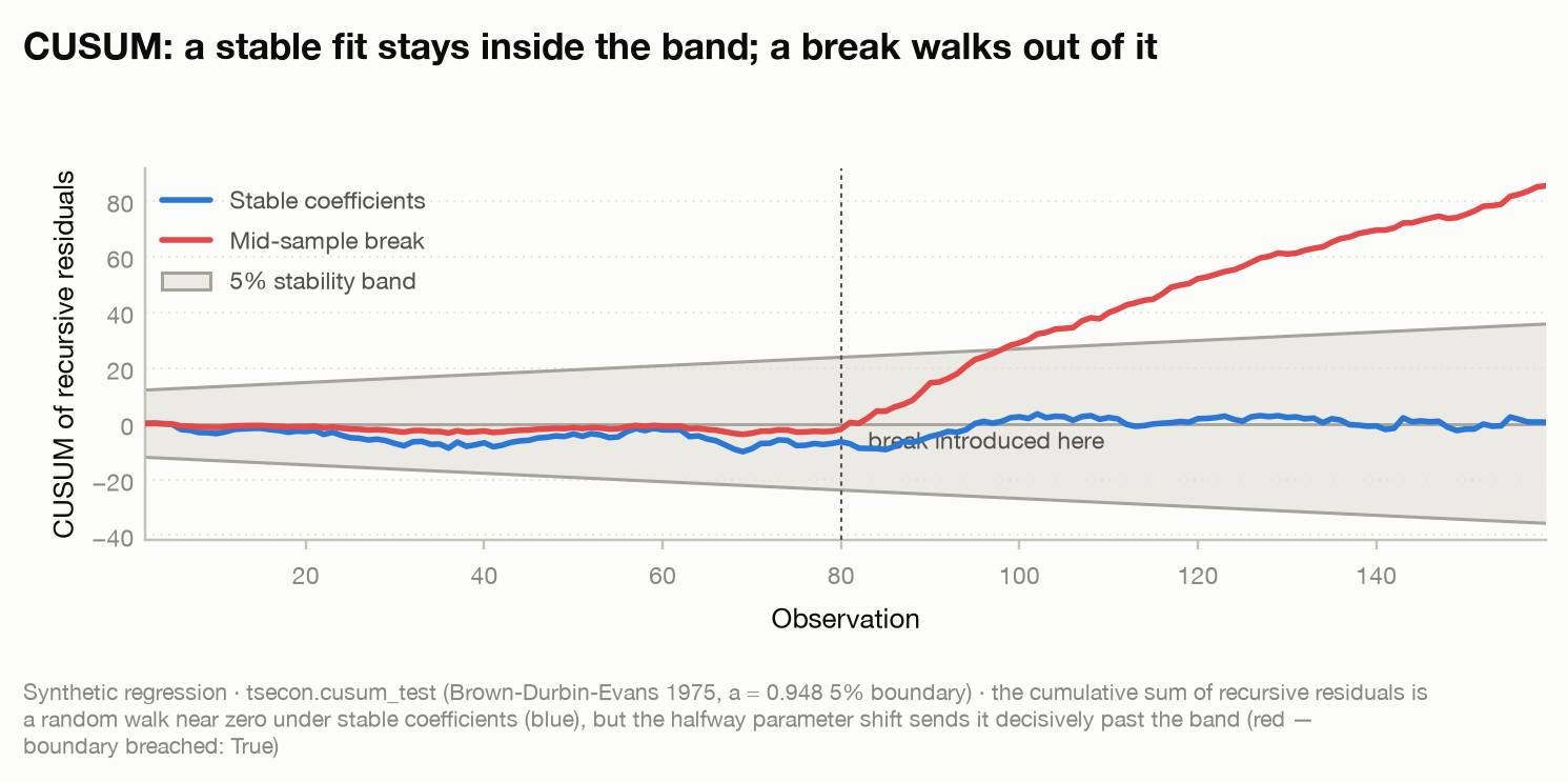
The stable fit (blue) stays inside the band; the series with a mid-sample break (red) crosses it decisively. See the specification-tests card.
Predictive regressions: IVX keeps its size near a unit root
Use case: regressing returns on a persistent, endogenous predictor (a dividend yield, a valuation ratio) breaks the OLS t-test — it over-rejects the harder the predictor's root approaches one. The IVX Wald test holds its size uniformly, up to and including an exact unit root.
fit = tsecon.predictive_regression(r, x)   # ols, stambaugh, and ivx views
fit["ivx"]["wald"], fit["ivx"]["pvalue"]   # the size-correct headline test
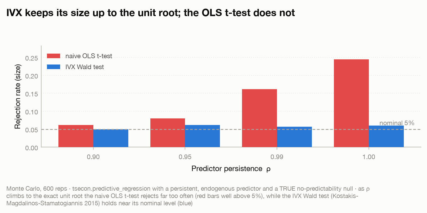
Under a true no-predictability null, the naive OLS t-test's rejection rate climbs
from 6% to 25% as ρ → 1, while the IVX Wald test stays near its nominal 5%. See
the predictive-regressions card.
Arbitrage-free Nelson-Siegel: one extra term
Use case: a plain Nelson-Siegel curve fits yields well but is not
arbitrage-free. Christensen-Diebold-Rudebusch keep the three loadings unchanged
and add a single closed-form adjustment term −A(τ)/τ that restores no-arbitrage.
adj = tsecon.afns_adjustment(maturities, sigma, decay=0.5)   # signed -A(tau)/tau
y_afns = y_ns + adj                                          # add to any NS fit
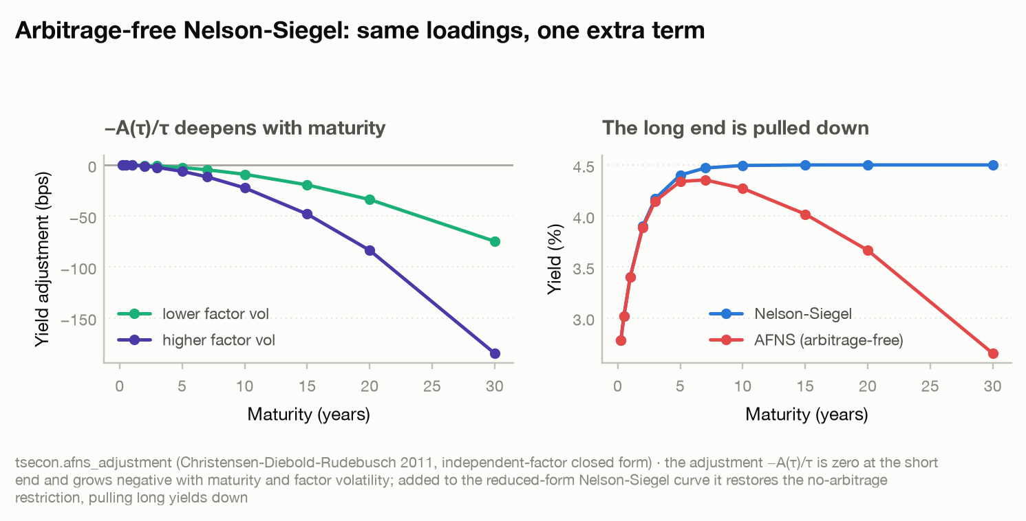
Left: the adjustment is zero at the short end and deepens with maturity and factor volatility. Right: added to the reduced-form curve it pulls the long end down — the no-arbitrage convexity effect. See the AFNS card.
DSGE-lite: the rational-expectations saddle path
Use case: solve a small linearized rational-expectations model to its policy rule and check determinacy. The Blanchard-Kahn count — unstable roots vs jump variables — decides whether the equilibrium is unique.
sol = tsecon.dsge_solve(A, B, C, n_predetermined=1)   # g, p, q, eigenvalue_moduli, verdict
sol["verdict"]   # "unique stable solution (1 unstable eigenvalue(s) = 1 jump variable(s))"
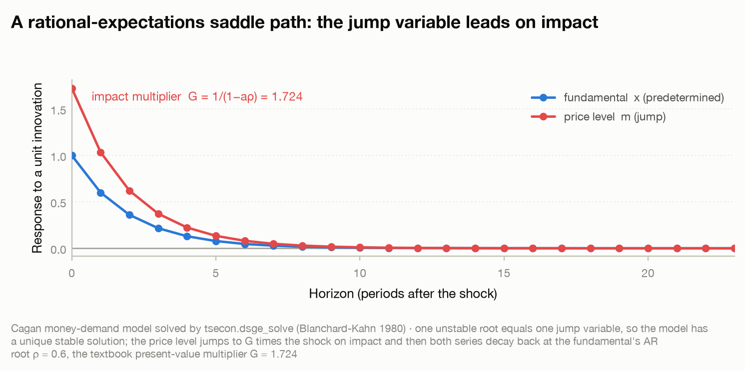
The Cagan money-demand model: the jump variable (price level) leads on impact by
the present-value multiplier G = 1/(1 − aρ), then both series revert at the
fundamental's AR root. See the DSGE card.
Spectral analysis: finding a cycle, and shared rhythm
Use case: how much of a series' variance sits at each frequency, and do two series share a cycle? The raw periodogram is a noisy, inconsistent estimate; Welch's segment-averaging turns it into a usable power spectral density, and magnitude-squared coherence measures frequency-by-frequency co-movement.
pg = tsecon.periodogram(x)     # raw PSD (freqs, psd) — matches scipy.signal to ~1e-15
wl = tsecon.welch(x)           # averaged, consistent PSD
co = tsecon.coherence(x, y)    # magnitude-squared coherence in [0, 1]
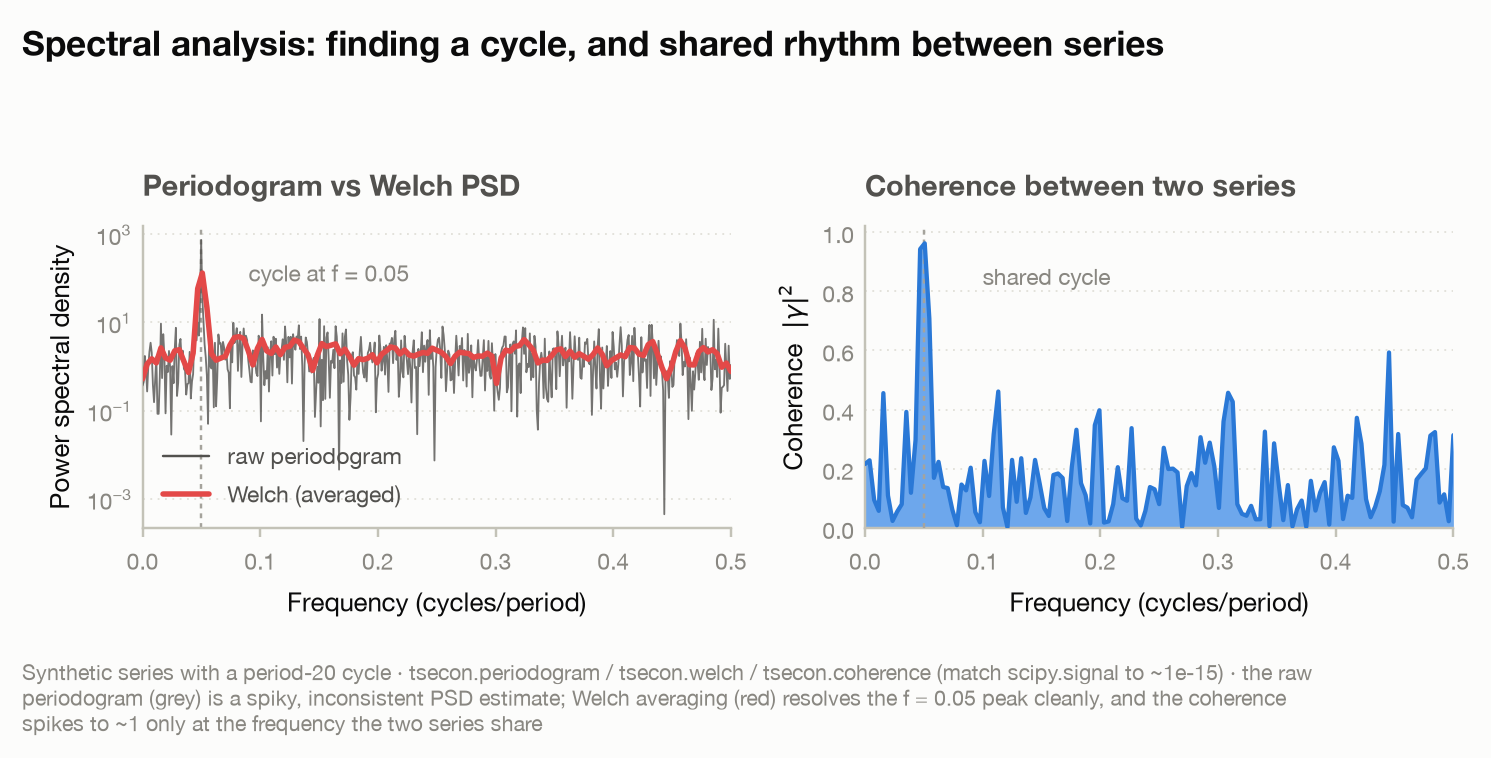
Left: the raw periodogram (grey) is spiky; Welch averaging (red) resolves the
f = 0.05 cycle cleanly. Right: coherence spikes to ~1 only at the frequency the
two series share. See the spectral card.