Chapter 10 — Bayesian Time Series
Part of The tsecon Guide to Time Series Econometrics. Chapters mirror the library's modules; code runs against the current Python API unless marked otherwise.
Prerequisites: OLS regression and the normal distribution; VARs and impulse responses (Chapter 6 material); a first look at state-space models and the Kalman filter helps for one section.
You will learn:
- How a prior and a likelihood combine into a posterior — worked once by hand with real numbers
- Why shrinkage is the whole point of Bayesian macroeconometrics, and what the Minnesota prior shrinks toward
- How the conjugate NIW-BVAR delivers the full posterior and a marginal likelihood in closed form, with no sampling at all
- What a Gibbs sampler actually does, when you need one, and how to tell whether a chain can be trusted
- How to read posterior impulse responses with credible bands — and how they genuinely differ from frequentist bands
The idea
You are a forecaster at a central bank. Your model is a VAR with seven variables — GDP growth, inflation, unemployment, a policy rate, and three more — with four lags of each. Count the parameters: each of the seven equations has an intercept plus 7 × 4 = 28 lag coefficients, so 29 per equation, 203 in total, before you even touch the error covariance matrix. Your data: quarterly observations since the late 1970s, roughly 200 usable rows.
Two hundred data points, two hundred parameters. Ordinary least squares will happily produce estimates — and they will be garbage. With that little data per parameter, OLS memorizes the sample's noise: coefficients on distant lags take large values with alternating signs, the fitted model looks wonderful in-sample, and the forecasts are terrible. This is not a software problem. It is a shortage of information, and no estimator can conjure information that the data do not contain.
But you are not actually ignorant. Before seeing a single observation you already know things about macroeconomic time series: most are highly persistent, so a variable's own recent past matters a lot; what happened three years ago matters much less than what happened last quarter; most cross-variable effects are modest. That knowledge is worth something — if only there were disciplined arithmetic for combining "what I knew before" with "what the data say."
That arithmetic is Bayes' rule. You express what you knew before as a probability distribution over the parameters — the prior. The data speak through the likelihood — the same object maximum likelihood uses, measuring how well each candidate parameter value explains what you observed. Multiplying the two and rescaling gives the posterior: a full probability distribution over the parameters after seeing the data.
Picture it as two bell curves drawn over the same axis. One is centered where your prior expects the parameter to be; the other is centered on what the data alone would estimate. The posterior is a third bell curve sitting between them — always closer to whichever of the two is narrower, that is, whichever carries more information. Lots of data and a vague prior: the posterior hugs the data. Little data and a sharp prior: the posterior stays near the prior. The compromise is automatic, optimal under the stated assumptions, and — this is the macro punchline — it shrinks wild data-driven estimates toward sensible values. In a 203-parameter VAR estimated on 200 observations, that shrinkage is not a nicety. It is the entire reason the model works.
There is a second, quieter payoff. The posterior is a genuine probability distribution over parameters, so questions practitioners actually ask — "what is the probability the impulse response is still positive after two years?" — have direct answers, with no appeal to imaginary repeated samples.
Bayes' rule, worked once by hand
Everything in this chapter is one formula applied with increasing ambition, so it pays to see the formula do its work once on a problem small enough to solve on paper.
Bayes' rule for a parameter \(\theta\) and data \(y\):
where \(p(\theta)\) is the prior, \(p(y \mid \theta)\) is the likelihood, \(p(\theta \mid y)\) is the posterior, and \(p(y) = \int p(y \mid \theta)\, p(\theta)\, d\theta\) — the marginal likelihood — is the rescaling constant that makes the posterior integrate to one. File that constant away: it looks like bookkeeping now, but it becomes the star of the show when we compare models.
Now the worked example. Suppose quarterly core inflation (annualized) is \(y_t \sim N(\mu, \sigma^2)\) with \(\sigma = 1\) known, and you want to learn the underlying mean \(\mu\). Your prior, reflecting a credible 2 percent inflation target: \(\mu \sim N(2,\ 0.5^2)\). You then observe \(T = 8\) quarters averaging \(\bar{y} = 3.4\).
For a normal likelihood with a normal prior, the posterior is again normal — the pair is called conjugate, meaning the prior family reproduces itself after updating — and the update has a closed form. Work in precisions (a precision is one over a variance; high precision = sharp information):
with prior mean \(\mu_0 = 2\) and prior variance \(\tau_0^2 = 0.25\). Plug in: prior precision \(1/0.25 = 4\); data precision \(8/1 = 8\); total \(12\). Posterior mean \(= (4 \times 2 + 8 \times 3.4)/12 \approx 2.93\); posterior standard deviation \(= \sqrt{1/12} \approx 0.29\).
Read the answer like an economist. The posterior mean is a precision-weighted average: the data contribute 8 of the 12 precision units, so the posterior sits two-thirds of the way from the prior toward the sample mean. Eight quarters of hot inflation moved you a long way off the 2 percent anchor — but not all the way, because eight observations is not much evidence. Collect 80 quarters instead and the data precision becomes 80: the prior is nearly irrelevant. That is the general pattern: the prior matters exactly when data are scarce — which, for macroeconomists with a few hundred quarterly observations, is always.
⚠ Common mistake. Treating a flat prior as "making no assumptions." A flat prior is itself a specific assumption — that a coefficient of 50 is as plausible as a coefficient of 0.5 — and in high-dimensional models flat priors produce the very overfitting Bayes exists to cure. Worse, flatness is not invariant: a prior flat on \(\theta\) is informative about \(1/\theta\) or \(\theta^2\). There is no assumption-free inference; the choice is between stated assumptions and hidden ones.
Why Bayes shines in macro: shrinkage is the point
Return to the parameter count. A VAR with \(n\) variables and \(p\) lags has \(k = 1 + np\) coefficients per equation and \(nk\) in total. At \(n = 7\), \(p = 4\): 203 coefficients. At \(n = 20\): 1,620. Bańbura, Giannone, and Reichlin (2010) estimate systems with over a hundred variables — tens of thousands of coefficients — on a few hundred observations. Frequentist OLS is not merely inefficient here; at some point \(X'X\) isn't even invertible.
The Bayesian escape is mechanical once you see it in the simplest case. Take a single regression \(y = X\beta + \varepsilon\) with \(\varepsilon \sim N(0, \sigma^2 I)\) and put the prior \(\beta \sim N(m, \tau^2 I)\). The posterior mean solves a penalized least squares problem:
Statisticians call the \(m = 0\) case ridge regression. The penalty weight \(\kappa\) is the ratio of noise variance to prior variance: a tight prior (small \(\tau^2\)) penalizes deviations from \(m\) heavily; a loose one barely at all. Adding \(\kappa I\) to \(X'X\) also fixes the invertibility problem — the posterior exists even with more parameters than observations.
Why does deliberately biasing your estimator toward \(m\) help? Bias–variance arithmetic. OLS is unbiased but, with 200 observations chasing 203 parameters, its variance is enormous — each estimate sits far from the truth, just in a random direction. Shrinkage accepts a small, controlled bias in exchange for a large variance reduction, and in mean-squared error the trade is overwhelmingly favorable when parameters are many and data are few. The prior is doing exactly what it did in the inflation example — anchoring the estimate where evidence is thin — just simultaneously, in hundreds of dimensions.
Two further advantages come along free. Bayesian inference is exact in finite samples: the posterior is the posterior whether \(T\) is 40 or 40,000, with no asymptotic approximations — welcome in a field where "large \(T\)" means two hundred. And the output is a full joint distribution over parameters, which propagates into forecast densities — fan charts with honest uncertainty — rather than bare point forecasts.
⚠ Common mistake. Judging a shrinkage estimator by in-sample fit. Shrinkage always fits the estimation sample worse than OLS — OLS is by construction the in-sample-fit champion. The gains appear out of sample, so evaluate with the tools of forecast evaluation (pseudo-out-of-sample exercises,
tsecon.dm_test), never with in-sample \(R^2\).
The Minnesota prior: shrink toward random walks
Shrinkage toward zero is the statistician's default, but macroeconomists can do better, because macro variables are not exchangeable coefficients — they are persistent time series. Robert Litterman and colleagues at the Federal Reserve Bank of Minneapolis proposed, in what is now universally called the Minnesota prior (Doan, Litterman, and Sims 1984; Litterman 1986), shrinking each equation of a VAR toward a univariate random walk: today's value equals yesterday's plus noise.
Concretely, the prior mean of every coefficient is zero except each variable's own first lag, which is centered at \(\delta = 1\) for levels data (random walk) or \(\delta = 0\) for growth rates and other stationary series (white noise). The prior variances then encode three beliefs through a small set of hyperparameters — parameters of the prior itself, best thought of as tightness dials:
- \(\lambda_1\) — overall tightness. Small \(\lambda_1\) (0.1–0.2 is typical): trust the random walk, shrink hard. Large: let the data speak. This is the single most consequential dial.
- \(\lambda_3\) — lag decay. Variances shrink with lag length like \(l^{-2\lambda_3}\), encoding "the distant past matters less"; \(\lambda_3 = 1\) is standard.
- \(\lambda_0\) — intercept looseness, set large (say 100) so the constant is essentially unrestricted.
- \(\sigma_j^2\) — not a dial but a scale correction: the residual variance of a univariate autoregression fit to variable \(j\), so that "one unit of coefficient" means the same thing whether the variable is an interest rate in percent or GDP in log levels. tsecon follows the AR(4)-with-intercept convention and documents it, because packages differ here and results are sensitive.
The library implements this prior in closed form (next section), but the idea runs today with tsecon.ols and one classic trick: a Gaussian prior is algebraically identical to a set of dummy observations — artificial data rows expressing the prior — appended to the real sample. OLS on the augmented data is the posterior mean. (This data-augmentation mechanic is exactly how production BVAR code implements Minnesota-family priors.) Here is an AR(12) — 13 parameters — on just 80 observations of a persistent series, shrunk toward a random walk with Minnesota-style lag decay:
import numpy as np
import tsecon

rng = np.random.default_rng(42)

# A persistent series (AR(1), phi = 0.97), T = 80 -- a short macro sample
T, p = 80, 12
y_full = np.zeros(T + p)
for t in range(1, T + p):
    y_full[t] = 0.97 * y_full[t - 1] + rng.standard_normal()

# AR(12) regression: 13 parameters from 80 observations
Y = y_full[p:]
X = np.column_stack([np.ones(T)] + [y_full[p - l : T + p - l] for l in range(1, p + 1)])

flat = tsecon.ols(Y, X, se_type="nonrobust")     # unrestricted OLS

# Minnesota-style prior: own lag 1 centered at 1, all else at 0,
# tightness lambda1 = 0.2, prior sd decaying like 1/lag (lambda3 = 1)
lam1  = 0.2
sigma = np.std(np.diff(y_full))                  # rough residual scale
mean  = np.r_[0.0, 1.0, np.zeros(p - 1)]         # random-walk center
tau   = np.r_[100.0, [lam1 / l for l in range(1, p + 1)]]  # loose intercept

# One dummy row per prior moment: OLS on the augmented system
# IS the posterior mean under the Gaussian prior
X_dummy = np.diag(sigma / tau)
y_dummy = (sigma / tau) * mean
post = tsecon.ols(np.r_[Y, y_dummy], np.vstack([X, X_dummy]), se_type="nonrobust")

print(flat["params"][1:].sum(), post["params"][1:].sum())    # persistence: similar
print(np.abs(flat["params"][5:]).max(), np.abs(post["params"][5:]).max())
With seed 42, both estimators agree on what is well identified — total persistence (the sum of lag coefficients: 0.90 flat vs. 0.89 shrunk). But OLS puts coefficients as large as 0.24 on lags 5 through 12, every one of which is truly zero: pure sample noise dressed up as dynamics. The shrunk estimate caps those same coefficients at 0.006. The prior spent its influence exactly where the data were uninformative and left the informative directions alone — shrinkage in one picture.
⚠ Common mistake. Shrinking toward \(\delta = 1\) regardless of the data's form. Centering the own first lag at 1 is a belief in random-walk levels. If you feed the model growth rates or other differenced data, that same center imposes extreme persistence the data do not have — use \(\delta = 0\) (shrink toward white noise). Getting this wrong quietly degrades every forecast the model makes.
The conjugate NIW-BVAR: a posterior without MCMC
Many people equate "Bayesian" with "MCMC and long waits." The workhorse BVAR needs none of that: with the right prior family, the posterior comes in closed form, exactly like the one-parameter inflation example. This closed form — implemented in the tsecon-bayes Rust crate and pinned by the golden fixture fixtures/bvar_niw.json, whose notation this section mirrors — is the computational backbone of everything else in this chapter.
Stack the VAR(\(p\)) as a multivariate regression: each row is \(y_t' = x_t' B + u_t'\), where \(x_t = (1, y_{t-1}', \dots, y_{t-p}')'\) collects the intercept and lags, \(B\) is the \(k \times n\) coefficient matrix (\(k = 1 + np\) regressors, \(n\) variables), and the errors are i.i.d. \(N(0, \Sigma)\) across the \(T\) usable rows. The natural-conjugate Normal-inverse-Wishart (NIW) prior (Kadiyala and Karlsson 1997) is
where the inverse-Wishart \(\mathcal{IW}\) is the standard prior for covariance matrices (\(S_0\) a scale matrix, \(v_0\) degrees of freedom — bigger \(v_0\), tighter prior), \(\otimes\) is the Kronecker product, and the Minnesota prior of the previous section supplies \(B_0\) (random-walk centers), the diagonal of \(\Omega_0\) (the \(\lambda\)-dial variances), \(S_0 = \mathrm{diag}(\sigma_1^2, \dots, \sigma_n^2)\), and \(v_0 = n + 2\). Conjugacy then delivers the posterior in four lines of matrix algebra — with \(X\) and \(Y\) the stacked regressor and data matrices:
Look at \(\bar{B}\): it is once again a precision-weighted average — prior precision \(\Omega_0^{-1}\) times prior mean, plus data precision \(X'X\) times the OLS information \(X'Y\), renormalized. The inflation example, grown up. Set \(\Omega_0^{-1} \to 0\) (a flat prior) and \(\bar{B}\) collapses to the OLS estimator; tighten the prior and it slides toward \(B_0\). The other two lines complete the picture: \(\bar{S}\) accumulates the prior scale, the data's sum of squares, and a correction for what the coefficient estimate already explained, while \(\bar{v} = v_0 + T\) simply counts the observations as added degrees of freedom.
Everything a practitioner wants then follows by direct simulation from these four moments — no Markov chains, no convergence worries:
- Coefficient uncertainty. Draw \(\Sigma \sim \mathcal{IW}(\bar{S}, \bar{v})\), then \(\mathrm{vec}(B) \mid \Sigma \sim N(\mathrm{vec}(\bar{B}), \Sigma \otimes \bar{\Omega})\). Each draw is exact and independent — two thousand of them take a fraction of a second through the Kronecker structure (the \(nk \times nk\) covariance is never formed).
- Impulse responses with uncertainty. Push each \((B, \Sigma)\) draw through the same companion-form recursion that
tsecon.var_irfuses, with a Cholesky factor of the drawn \(\Sigma\); the collection of IRF surfaces is the posterior distribution of impulse responses. - Forecast fan charts. For each draw, simulate the VAR forward with fresh shocks. Crucially, this integrates parameter uncertainty into the predictive density — plugging in the posterior-mean parameters instead and simulating only shocks understates forecast uncertainty, a pervasive error in forecast-evaluation code.
The whole pipeline is fast enough to re-estimate hundreds of times in a recursive out-of-sample exercise, which is exactly how BVAR forecasting papers are validated.
The same conjugacy yields the marginal likelihood \(p(Y)\) in closed form — a matrix-variate-\(t\) density (Kadiyala and Karlsson 1997):
with \(\Gamma_n\) the multivariate gamma function. This number is the evidence: the probability the model-plus-prior assigned to the data you actually saw, with all parameters integrated out. Its practical use is immediate — the tightness dials \(\lambda_0, \lambda_1, \lambda_3\) change \(\Omega_0\), so you can score hyperparameter settings by their marginal likelihood and let the data pick the dials. That one observation powers the hierarchical methods two sections ahead.
This runs today: tsecon.bvar_fit returns the closed-form NIW posterior and its log marginal likelihood, and tsecon.bvar_irf_draws pushes each posterior draw through the same companion-form recursion tsecon.var_irf uses to build the impulse-response draws for credible bands — both backed by the MinnesotaNiwPrior / NiwPosterior Rust core and pinned to the golden fixture above. These data are growth rates, so the own first lag shrinks toward white noise (delta=0), not a random walk:
import json, numpy as np, tsecon

data = np.array(json.load(open("fixtures/bvar_niw.json"))["data"])   # 202 x 3 macro growth rates

post = tsecon.bvar_fit(data, lags=2, lambda0=100.0, lambda1=0.2,
                       lambda3=1.0, delta=0.0)
post["posterior_mean_coefs"]        # posterior-mean coefficients B-bar, k x n
post["sigma_posterior_mean"]        # posterior-mean error covariance, n x n
post["log_marginal_likelihood"]     # the evidence -- tune lambda1 with it   (-861.57)

# Posterior IRF draws [draw][h][response][shock] -- the raw material for credible bands
irf = tsecon.bvar_irf_draws(data, lags=2, horizon=16, n_draws=2000, seed=0)
⚠ Common mistake. Inverse-Wishart parameterization mismatches. "\(\Sigma \sim \mathcal{IW}(S, v)\)" means the scale convention in some papers and packages (prior mean \(S/(v - n - 1)\)) and the rate convention (\(S^{-1}\) in the density) in others, with degrees-of-freedom offsets that differ too. This is the single most common reason your BVAR "doesn't replicate" a published result. tsecon uses the scale convention — mean \(S/(v-n-1)\), matching R
BVAR, BEAR, and the Giannone-Lenza-Primiceri replication code — and says so in the docs; check the convention before comparing numbers across packages.
When you do need sampling: Gibbs, chains, and the simulation smoother
Conjugacy is a special deal: it holds because the NIW prior's Kronecker structure matches the likelihood's. Ask for more — prior variances that differ freely across equations, stochastic volatility, time-varying coefficients — and the posterior stops having a name. You can still write \(p(\theta \mid y) \propto p(y \mid \theta)\, p(\theta)\); you just cannot integrate it analytically, and with hundreds of dimensions, numerical integration on a grid is hopeless.
Markov chain Monte Carlo (MCMC) solves this with a change of goal: stop trying to compute the posterior and instead draw samples from it. Any posterior quantity — means, quantiles, the probability an IRF is positive at horizon 8 — is then just an average over draws.
The tool of choice in BVAR-land is the Gibbs sampler (Gelfand and Smith 1990). Split the parameters into blocks — say coefficients \(B\) and covariance \(\Sigma\). You cannot draw from \(p(B, \Sigma \mid y)\) jointly, but each block's full conditional — its distribution given the data and the current value of the other block — is often a standard distribution. So iterate:
Each draw depends only on the previous one: the sequence \((B^{(s)}, \Sigma^{(s)})\) is a Markov chain. The remarkable theorem is that this chain's long-run (stationary) distribution is exactly the joint posterior. The intuition: if the current draw already came from the posterior, drawing one block from its exact conditional leaves the joint distribution undisturbed — the posterior is a fixed point of the update — and under mild conditions the chain converges to that fixed point from any starting value. So run it long enough and the draws — after discarding an initial burn-in during which the chain forgets its arbitrary starting point — behave like (correlated) samples from \(p(B, \Sigma \mid y)\), and their averages converge to posterior expectations. No algorithm worship needed: a Gibbs sampler is just "alternate between two conditional regressions until the pair settles into its equilibrium distribution." When a block's conditional is nonstandard, a Metropolis-Hastings step (propose a move, accept it with a probability that keeps the posterior stationary; Chib and Greenberg 1995) fills the gap inside the same loop.
Two points of craft before the diagnostics. Burn-in is for forgetting the starting point, nothing more — if a chain has not converged, doubling the burn-in is a hope, not a fix; the diagnostics in the next section are the arbiter. And thinning (keeping every \(k\)-th draw to reduce autocorrelation) mostly wastes information: correlated draws still contribute to posterior averages, so keep them all unless memory forces your hand, and let the effective sample size account for the correlation honestly.
For time series the essential Gibbs block is the simulation smoother. Time-varying-parameter and stochastic-volatility models are state-space models: the drifting coefficients (or log-volatilities) are an unobserved path \(\alpha_1, \dots, \alpha_T\), thousands of correlated unknowns. The Carter-Kohn forward-filter backward-sampling (FFBS) algorithm (Carter and Kohn 1994; Frühwirth-Schnatter 1994) draws the entire path in one shot: run the Kalman filter forward to get the filtered moments, then sample backward from \(T\) to 1, each state conditioned on the one just drawn after it. The result is one exact joint draw of the whole trajectory — the bridge between Chapter 5's state-space machinery and everything Bayesian that moves over time. You have already seen what such a draw is a draw of:
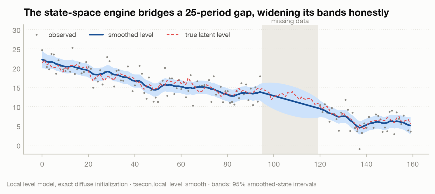
The smoothed mean and band from the local-level model (tsecon.local_level_smooth) summarize the distribution of paths; an FFBS draw is one random path from that distribution, wiggling inside the band — wider where data are missing. Inside a Gibbs loop, the sampler alternates "draw the path given the parameters (FFBS)" with "draw the parameters given the path (conjugate regressions)". tsecon's Carter-Kohn implementation (FfbsSampler in the tsecon-bayes crate) handles the singular state covariances of companion-form models with rank-aware pseudo-inverses — a classic crash-or-silently-wrong site in home-rolled code — and draws all randomness through the same Philox counter-based generator as tsecon.philox_uniforms, keyed by (seed, chain, draw, block), so multi-chain runs are bitwise reproducible at any thread count.
⚠ Common mistake. "The chain ran, so it worked." A Gibbs sampler with a subtly wrong conditional — a mis-ordered block, a stale conditioning value — still produces smooth traces and plausible-looking posteriors; they are simply posteriors of the wrong model. This is not hypothetical: the block ordering in Primiceri's (2005) canonical TVP-VAR sampler was wrong for a decade until Del Negro and Primiceri (2015) corrected it, and the Carriero-Clark-Marcellino (2019) large-BVAR algorithm needed a 2022 corrigendum. tsecon ships only the corrected samplers and runs Geweke (2004) joint-distribution tests in CI, because eyeballs cannot catch this class of bug.
Trust, but verify: convergence diagnostics
MCMC output is only as good as the chain's behavior, and two failure modes matter. The chain may not have converged — it is still drifting toward the posterior's bulk, so early draws contaminate your averages. Or it mixes slowly — successive draws are so correlated that 10,000 of them carry the information of 200 independent ones. Both are invisible in a table of posterior means. Modern practice (Vehtari, Gelman, Simpson, Carpenter, and Bürkner 2021) diagnoses them with two numbers, and tsecon computes both to numerical agreement with ArviZ and the R posterior package.
Rank-normalized split \(\widehat{R}\) answers "did the chains converge — and to the same place?" Run several chains (four is the default) from deliberately scattered starting points, split each in half so a still-trending chain betrays itself as disagreement between its own halves, rank-normalize the draws so heavy tails cannot break the variance calculations, and compare within-chain variance \(W\) to between-chain variance:
If every chain explores the same distribution, between and within variation match and \(\widehat{R} \to 1\). The working threshold: be suspicious above 1.01 — a far stricter bar than the 1.1 of older practice, and one that older, non-split, non-rank-normalized \(\widehat{R}\) versions frequently pass while the sampler is failing.
Effective sample size (ESS) answers "how much information do the draws contain?" With autocorrelation \(\rho_t\) at lag \(t\) along the chain,
for \(M\) chains of \(N\) draws. A slowly mixing chain has \(\rho_t\) near 1 for many lags and an ESS a tiny fraction of \(MN\). Vehtari et al. distinguish bulk ESS (reliability of central summaries like posterior means and medians) from tail ESS (reliability of the 5% and 95% quantiles — precisely the credible-band endpoints macro papers report). Chains routinely have healthy bulk ESS and poor tail ESS; if you report bands, check the tail number. A rule of thumb: want ESS above ~400 before quoting two-digit summaries.
The pre-flight checklist, then, for any MCMC output you intend to publish:
- Run at least 4 chains from overdispersed starting points — convergence claims from one chain are unfalsifiable.
- Require \(\widehat{R} < 1.01\) for every quantity you report, not just the headline parameters.
- Check bulk ESS before quoting means and tail ESS before quoting credible-band endpoints; treat values below a few hundred as "collect more draws."
This runs today: tsecon.mcmc_diagnostics returns all three numbers in one call from a (chains, draws) array of one scalar quantity — the Rust implementations (rhat_rank, ess_bulk, ess_tail) validated against ArviZ:
import numpy as np, tsecon

# 4 chains x 500 draws of one reported scalar (e.g. the horizon-8 IRF ordinate)
rng = np.random.default_rng(0)
chains = rng.standard_normal((4, 500))

diag = tsecon.mcmc_diagnostics(chains)
diag["rhat"]        # rank-normalized split R-hat        (want < 1.01)
diag["ess_bulk"]    # effective draws for means/medians
diag["ess_tail"]    # effective draws for the 5%/95% quantiles
⚠ Common mistake. Running one long chain and eyeballing its trace plot. A single chain stuck in one mode of a multimodal posterior — routine in Markov-switching models — produces a beautiful, stable, utterly misleading trace. \(\widehat{R}\) can only detect this from multiple chains started at overdispersed points; that is why tsecon's samplers default to four chains and compute \(\widehat{R}\) whether or not you ask. Diagnostics are also per quantity: a converged intercept says nothing about the horizon-12 IRF, so compute ESS for every function of draws you report.
Letting the data set the dials: hierarchical priors, TVP, and stochastic volatility
Three extensions dominate modern applied work, and all three are conceptually small steps from what you now know.
Hierarchical priors: the data choose the tightness. The Minnesota \(\lambda_1\) was, for decades, set by folklore (0.2 and pray) or by grid search on forecast RMSE. Giannone, Lenza, and Primiceri (2015) made the obvious-in-retrospect move: if \(\lambda\) is unknown, treat it Bayesianly — put a prior (a hyperprior) on the hyperparameters and use Bayes' rule one level up:
The magic ingredient is one you already have: \(p(Y \mid \lambda)\) is exactly the closed-form NIW marginal likelihood, evaluated at the prior that \(\lambda\) implies. Estimating the dials costs a low-dimensional sampler (or just an optimizer, for the empirical-Bayes mode) wrapped around a formula — and it works so well that "GLP" is now the default prior in serious BVAR forecasting. One implementation subtlety with teeth: every term of the marginal likelihood that depends on \(\lambda\) must be kept — the "constants" people drop when they only ever compare parameters within one model are not constant across priors, and dropping them silently corrupts the hyperparameter posterior.
tsecon ships the empirical-Bayes (ML-II) mode today as bvar_hierarchical: it maximizes the closed-form marginal likelihood over the tightness lambda1, then refits the conjugate posterior at the optimum — a drop-in bvar_fit that tunes its own shrinkage.
import json, numpy as np, tsecon

bh_data = np.array(json.load(open("fixtures/var.json"))["data_100dlog_gdp_cons_inv"])
h = tsecon.bvar_hierarchical(bh_data, lags=2, optimize="lambda1")
print("selected lambda1:", round(h["lambda1_opt"], 4),
      " log-ML at optimum:", round(h["log_marginal_likelihood"], 4))
print("log-ML at the conventional lambda1 = 0.2:", round(h["lambda1_fixed_log_ml"], 4))

# On a short, persistent sample the data-chosen tightness moves off 0.2 and the
# marginal likelihood improves materially over the folklore default.
rng_bh = np.random.default_rng(1)
Ys = np.zeros((60, 4))
for t in range(1, 60):
    Ys[t] = 0.8 * Ys[t - 1] + 0.3 * rng_bh.standard_normal(4)
hs = tsecon.bvar_hierarchical(Ys, lags=3, optimize="lambda1")
print("short sample: selected lambda1 =", round(hs["lambda1_opt"], 4),
      " log-ML gain over fixed 0.2 =",
      round(hs["log_marginal_likelihood"] - hs["lambda1_fixed_log_ml"], 3))
selected lambda1: 0.1944  log-ML at optimum: -861.5642
log-ML at the conventional lambda1 = 0.2: -861.5704
short sample: selected lambda1 = 0.3032  log-ML gain over fixed 0.2 = 3.563
On the long fixture sample the evidence is nearly flat in lambda1: the ML-II optimum (0.194) sits a whisker from the folklore 0.2 and barely improves the marginal likelihood — the data have little to say about the dial. On the short, persistent 4-variable sample the picture flips: the data pull the tightness up to 0.30 and buy a 3.6-log-point improvement, exactly the regime where letting the evidence set the dial matters. Pass optimize="lambda1+lambda3" to also tune the lag-decay rate, or hyperprior="glp" for the GLP Gamma hyperprior (MAP-II rather than pure ML-II); the fully sampled hierarchical posterior with credible bands on lambda remains a Module 05 roadmap item.
Spike-and-slab selection: let the data zero out coefficients. Shrinkage
pulls every coefficient toward the prior by a common dial; stochastic search
variable selection (SSVS; George, Sun and Ni 2008) instead asks, one
coefficient at a time, whether it belongs in the model at all. Each coefficient
gets a two-component prior — a narrow spike \(N(0,(c_0\tau)^2)\) pinning it near
zero and a wide slab \(N(0,(c_1\tau)^2)\) letting the data speak — with a latent
0/1 indicator switching between them, and a Gibbs sampler draws the indicators
alongside the coefficients. The fraction of draws in which a coefficient is
"in" is its posterior inclusion probability: a soft, honest selector where
the LASSO gives a hard threshold, and a full posterior where the LASSO gives a
point. It is the Bayesian answer to a sparse VAR — most distant lags and
cross-effects truly zero — and tsecon.bvar_ssvs ships it today. On a sparse
VAR(2) it recovers the pattern without a single hard cutoff:
import numpy as np, tsecon

rng = np.random.default_rng(0)
n, T, p = 3, 300, 2
A1 = np.array([[0.5, 0.0, 0.0], [0.3, 0.4, 0.0], [0.0, 0.0, 0.6]])   # sparse
A2 = np.array([[0.0, 0.0, 0.0], [0.0, 0.0, 0.0], [0.0, 0.0, 0.2]])   # sparser
c = np.array([0.2, -0.1, 0.0])
Y = np.zeros((T + 50, n))
for t in range(2, T + 50):
    Y[t] = c + A1 @ Y[t - 1] + A2 @ Y[t - 2] + 0.5 * rng.standard_normal(n)
Y = Y[50:]

res = tsecon.bvar_ssvs(Y, lags=2, n_draws=4000, burn=1000, seed=1, n_chains=2)
inc = np.asarray(res["inclusion_prob"])    # (1+pK) x n; intercept row pinned to 1
print(np.round(inc, 2))
print("mean model size:", round(res["diagnostics"]["mean_model_size"], 2),
      "slopes (true: 5)  R-hat:", round(res["diagnostics"]["rhat"], 4))
[[1.   1.   1.  ]
 [1.   1.   0.11]
 [0.36 1.   0.08]
 [0.07 0.16 1.  ]
 [0.12 0.21 0.08]
 [0.09 0.09 0.09]
 [0.09 0.22 0.84]]
mean model size: 6.59 slopes (true: 5)  R-hat: 1.0043
Every one of the five true non-zero coefficients earns an inclusion probability
from 0.84 to 1.0 — the weakest, the 0.2 second-lag term, still clears 0.8 —
while the true zeros stay at 0.36 or below. The one SSVS wrinkle to watch: the
discrete inclusion indicators are highly autocorrelated, so their effective
sample size lags the continuous parameters' badly (check ess_bulk) — run long,
and diagnose with multiple chains as always. The horseshoe and Normal-Gamma
global-local shrinkage families that SSVS competes with in forecasting horse
races are the frontier, below.
Time-varying parameters (TVP). Was the Fed's inflation response the same in 1975 as in 2005? A TVP-VAR answers by letting coefficients follow random walks, \(\beta_t = \beta_{t-1} + \eta_t\) — a state-space model estimated by Gibbs with FFBS drawing the coefficient paths (Cogley and Sargent 2005; Primiceri 2005, as corrected by Del Negro and Primiceri 2015). Conceptually: the Minnesota prior shrinks coefficients toward a point; a TVP prior shrinks changes in coefficients toward zero, with the state-innovation variance controlling how much history is allowed to bend. One documented choice deserves daylight: many TVP implementations discard coefficient draws whose implied VAR is explosive (following Cogley and Sargent). That truncation is a change of prior, not a numerical detail — it alters the posterior and the marginal likelihood, and near unit roots it can silently reject almost every draw. tsecon's roadmap makes it an explicit, reported option rather than a hidden default.
Stochastic volatility (SV). Macro residual variances are wildly non-constant — the Great Moderation, 2008, March 2020. SV lets each shock's log-variance follow its own random walk, sampled with the Kim-Shephard-Chib (1998) mixture trick that turns the nonlinear volatility model into a conditionally linear one FFBS can handle. In forecasting exercises SV is often worth more than any other single extension: it is what lets a fan chart widen in turbulent times and narrow in calm ones.
⚠ Common mistake. Two, both documented failure modes. TVP overfitting: a loose prior on state-innovation variances lets coefficient paths wiggle to absorb what is really noise, producing dramatic "evolving transmission" narratives from an overfit model — modern practice shrinks the state variances themselves (Frühwirth-Schnatter and Wagner 2010). SV ordering dependence: the standard Cholesky-based multivariate SV makes the reduced-form covariance itself depend on the order you list the variables — an econometric artifact, not a numerical one. Reorder GDP and inflation and your volatility estimates change. Order-invariant alternatives (common SV; the Chan-Koop-Yu 2024 specification) exist; tsecon's roadmap ships them alongside the standard form with a warning attached.
Comparing models and reading the bands
Model comparison. The marginal likelihood earns its keep here. For models \(M_1, M_2\) the Bayes factor
updates prior model odds into posterior odds. Because each \(p(Y \mid M_i)\) integrates over the model's parameters, the Bayes factor has a built-in Occam's razor: a flexible model spreads its prior probability over many possible datasets and is penalized on the ones it didn't need the flexibility for — no ad hoc complexity correction required. A useful reading scale (after Kass and Raftery 1995): a log Bayes factor \(\ln BF_{12}\) between 0 and 1 is "barely worth mentioning," 1–3 positive, 3–5 strong, above 5 very strong. Since marginal likelihoods of BVARs differ by hundreds of log points across sensible tightness settings — the fixture's 3-variable golden case pins \(\ln p(Y) = -861.57\) for one specific prior — the evidence usually speaks clearly.
With closed-form NIW marginal likelihoods, comparison is cheap enough to run over lag lengths, variable sets, and priors simultaneously, and Bayesian model averaging — weighting each model's forecast by its posterior model probability — often beats every individual model. Honesty requires two warnings. First, for models estimated by MCMC with latent states (SV, TVP), the marginal likelihood is genuinely hard: the popular harmonic-mean estimator has infinite variance and should never be used (tsecon refuses to ship it), and naive Chib-style estimates built on the conditional-on-states likelihood are biased (Chan and Grant 2015). Second, Bayes factors are sensitive to prior scales in a way posteriors are not — the Lindley paradox: against a point null, diffusing a prior toward flatness drives the Bayes factor toward the null regardless of the data.
⚠ Common mistake. Computing Bayes factors under improper (infinite-mass) or arbitrarily vague priors. Improper priors leave the marginal likelihood defined only up to an arbitrary constant, so the resulting Bayes factor is meaningless; very vague proper priors are nearly as bad via Lindley. Parameter inference tolerates vague priors; model comparison does not. Use proper, deliberately scaled priors — or compare models on out-of-sample density forecasts instead.
Credible bands vs. confidence bands. A Bayesian credible band around an impulse response means what everyone secretly wants bands to mean: given the data, the model, and the prior, the IRF lies inside with 90% probability. A frequentist confidence band means something else: the band-constructing procedure, applied over hypothetical repeated samples, would trap the true fixed IRF 90% of the time — for the one dataset you have, the realized band either contains the truth or doesn't, and no probability attaches to it. Concretely, the sentence "there is a 92% chance output is still below baseline two years after the shock" is licensed by a posterior (count the draws) and by nothing in the frequentist toolkit; the sentence "under repeated sampling this procedure rarely misleads" is the frequentist guarantee, and the Bayesian band offers it only asymptotically. In large samples with vague priors the two often nearly coincide (the Bernstein–von Mises phenomenon), which is why people conflate them. They diverge exactly where Bayes is being useful: with informative priors and short samples, credible bands are narrower and shifted toward the prior — tighter dials, tighter bands. That is a feature when the prior is defensible and quiet assumption-laundering when it isn't, which is why hierarchical tightness selection and prior-sensitivity checks belong in the reporting standard. For orientation, here is the frequentist point-estimate IRF grid from the gallery — the object a BVAR replaces with a full posterior distribution of IRF surfaces, one per draw, summarized by quantile bands:
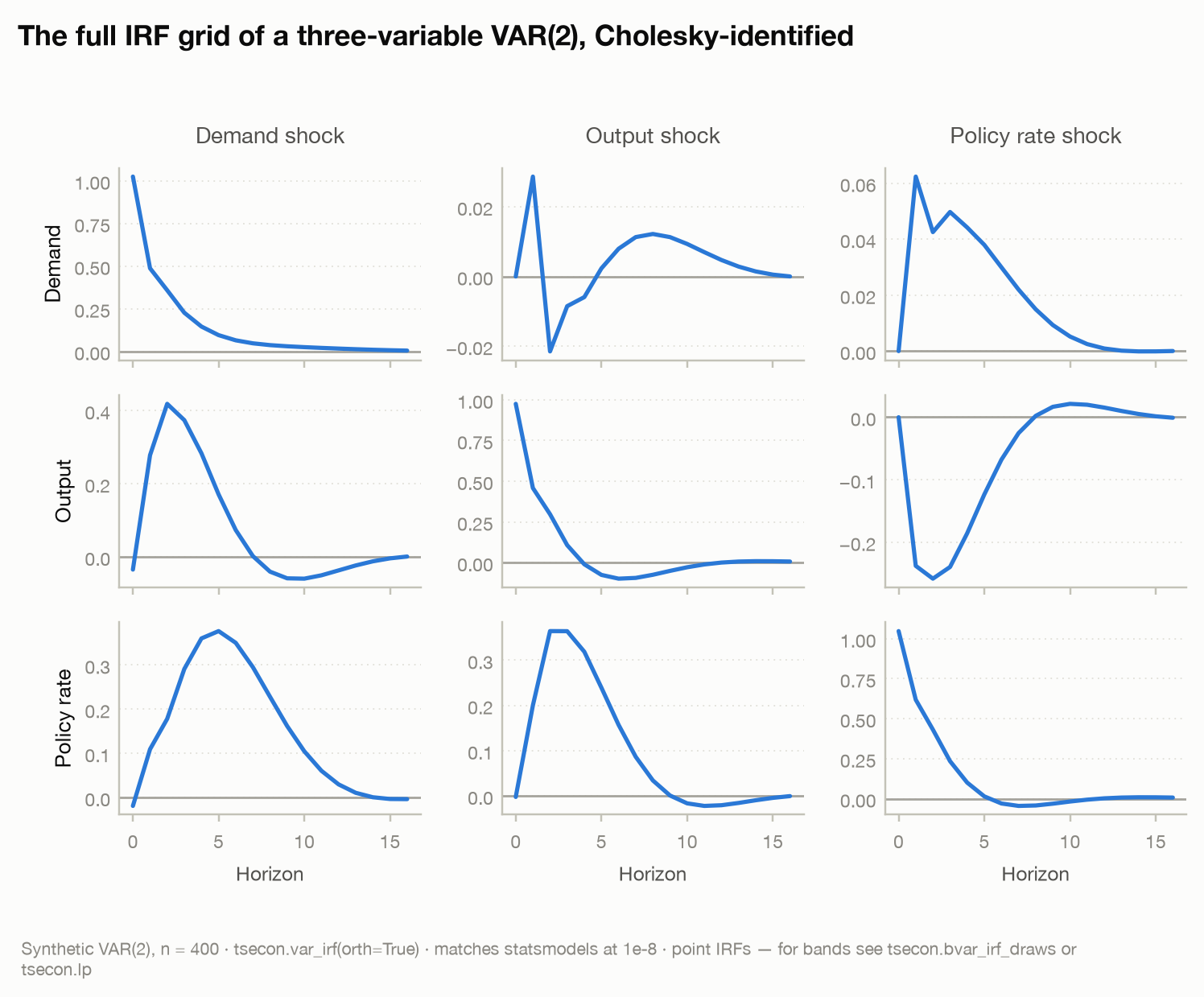
Runnable today as the frequentist baseline (and the natural sanity check on any BVAR you fit — with loose priors, the posterior median IRF should approximately reproduce it):
import json, numpy as np, tsecon

data = np.array(json.load(open("fixtures/var.json"))["data_100dlog_gdp_cons_inv"])  # 202 x 3

irf = tsecon.var_irf(data, lags=2, horizon=16)   # [h][response][shock]
fc  = tsecon.var_forecast(data, lags=2, steps=8) # point + intervals
One final honesty note that applies to both paradigms: the bands macro papers plot are almost always pointwise — a separate 90% statement at each horizon — so the probability that the entire IRF path stays inside is well below 90%. Joint (simultaneous) bands are wider; see the frontier.
The frontier
The state of the art, and where the Module 05 roadmap is headed:
- Hierarchical priors as the default. Giannone, Lenza, and Primiceri (2015) ended the fixed-\(\lambda\) era; the follow-on "prior on the long run" (Giannone, Lenza, and Primiceri 2019) disciplines long-horizon behavior through beliefs about great ratios rather than ad hoc dummy observations. The first of the pair is no longer frontier — it ships as
bvar_hierarchical, the ML-II/MAP-II selection this chapter ran above; the fully sampled \(\lambda\) posterior and the prior on the long run remain roadmap items with the authors' replication files as validation gates. - Correctness as a differentiator. The field's most-cited samplers shipped wrong: Primiceri (2005) (corrected by Del Negro and Primiceri 2015) and Carriero-Clark-Marcellino (2019) (corrigendum: Carriero, Chan, Clark, and Marcellino 2022) — and uncorrected code still circulates. tsecon implements only corrected samplers, and the correctness evidence is specific rather than sweeping: the FFBS simulation smoother carries a Geweke (2004) "getting it right" joint-distribution test in the Rust suite, and the SSVS Gibbs sampler behind
bvar_ssvsis graded by seeded Monte-Carlo support recovery, bitwise seed reproducibility, and multi-chain convergence. Simulation-based calibration (Talts et al. 2018) across every sampler is the roadmap's bar, not today's. - Scale. Large conjugate BVARs (Bańbura, Giannone, and Reichlin 2010) made 100-variable systems routine; Chan's (2022) asymmetric conjugate prior restores genuine cross-variable Minnesota shrinkage with a closed-form marginal likelihood at that scale. Beyond MCMC entirely: variational Bayes for huge systems (honest caveat — VI understates posterior variance) and sequential Monte Carlo for multimodal posteriors (Herbst and Schorfheide 2014), both embarrassingly parallel and natural fits for the Rust core.
- Global-local shrinkage. The horseshoe prior (Carvalho, Polson, and Scott 2010) and Normal-Gamma/Dirichlet-Laplace families shrink adaptively — hard on noise, gently on signal — and win several BVAR forecasting horse races; the roadmap puts them behind one "shrinkage family" interface so users can horse-race priors. None of that family is callable yet — the shipped sparse-VAR route is the spike-and-slab
bvar_ssvs. - Post-2020 volatility. COVID observations broke naive SV; current practice uses outlier-robust SV (Carriero, Clark, Marcellino, and Mertens 2022) or explicit pandemic volatility scaling (Lenza and Primiceri 2022) — "downweight, don't drop."
- Honest uncertainty statements. Joint credible bands for IRFs (Inoue and Kilian 2022) fix the pointwise-band miscoverage above and are still roadmap; the rank-normalized diagnostics (Vehtari et al. 2021) are not — they ship in Python as
mcmc_diagnostics, matching ArviZ and Rposteriornumerically. - Open problems. Marginal likelihoods for latent-state models remain expensive and fragile (Chan and Grant 2015 documents the biases in common shortcuts); order dependence in Cholesky-based multivariate SV has fixes but no consensus default; TVP models still walk a knife edge between missing genuine change and hallucinating it; and the informativeness of "agnostic" priors in set-identified structural models (Baumeister and Hamilton 2015) — owned by the identification module — remains the sharpest active debate in Bayesian macro.
Which method when
| Situation | Reach for | Because |
|---|---|---|
| Forecasting VAR, 3–10 variables, typical macro sample | bvar_fit — the conjugate Minnesota/NIW-BVAR, tightness compared via its log_marginal_likelihood |
Closed form — fast, no convergence worries; shrinkage cures overparameterization |
| Choosing the tightness dials | bvar_hierarchical — GLP empirical-Bayes / ML-II |
The data pick \(\lambda\) by maximizing the closed-form evidence; folklore values retire |
| Sparse VAR — let the data zero out coefficients | bvar_ssvs — spike-and-slab stochastic search |
Posterior inclusion probabilities select which lags/cross-effects survive; a soft LASSO with a full posterior |
| 20–130 variables | Large conjugate BVAR, shrinkage tightened with dimension — roadmap; bvar_fit is the same prior at the scales above |
Bańbura et al. (2010): beats factor models; conjugacy keeps it feasible |
| Prior must differ freely across equations | Independent Normal-Wishart + Gibbs — roadmap | The Kronecker restriction of the conjugate form is the price of closed forms |
| Suspected drift in dynamics (policy regimes, structural change) | TVP-BVAR via FFBS, with shrinkage on state variances — roadmap (the FFBS smoother exists in the Rust crate, unbound); markov_switching_ar is the shipped discrete-regime alternative |
Random-walk coefficients; shrinkage prevents hallucinated time variation |
| Volatility clustering, crisis samples, fan charts | BVAR-SV (order-invariant variant if available) — roadmap; univariate SV-style volatility ships as gas_volatility/dcs_local_level (Chapter 6) |
Constant-variance bands mislead in both calm and turbulent periods |
| Comparing lag lengths, priors, variable sets | bvar_fit's log_marginal_likelihood differenced across specifications (Bayes factors); BMA is roadmap |
Evidence integrates out parameters; automatic Occam penalty |
| Any MCMC output, before believing it | mcmc_diagnostics on 4 chains — rank-normalized split \(\widehat{R}\) < 1.01, bulk and tail ESS |
Single chains and trace-plot eyeballing miss stuck and slow-mixing samplers |
| Reporting IRF uncertainty from a posterior | bvar_irf_draws, then your own per-horizon quantiles, labeled pointwise vs. joint |
Credible bands answer the probability question people actually ask |
| Suspected multimodal posterior (regime switching) | Many dispersed chains or SMC, never a single Gibbs run | Gibbs chains get trapped in one mode and look perfectly converged |
| Just need point IRFs and forecasts today | tsecon.var_irf, tsecon.var_forecast |
Frequentist workhorse, available now — and the sanity check on any BVAR |
What tsecon implements today
Available now in Python (import tsecon) — the pieces this chapter's runnable code used:
tsecon.ols— the shrinkage demonstration via dummy observations (se_type="nonrobust"|"hc0"|"hc1"|"hc2"|"hc3"|"hac"; the leverage-correctedhc2/hc3rungs are the ones that matter at small \(n\) — see Chapter 3)tsecon.bvar_fit— the conjugate Minnesota/NIW-BVAR: closed-form posterior-mean coefficients \(\bar{B}\), posterior-mean \(\Sigma\), and the matrix-variate-\(t\) log marginal likelihood (backed by theMinnesotaNiwPrior/NiwPosteriorRust core)tsecon.bvar_hierarchical— empirical-Bayes / ML-II tightness selection (Giannone-Lenza-Primiceri 2015): maximizes that same marginal likelihood overlambda1(optionallylambda1+lambda3, or MAP-II under the GLP Gamma hyperprior), then refits the posterior at the optimumtsecon.bvar_ssvs— spike-and-slab stochastic-search variable selection (George-Sun-Ni 2008): a four-block Gibbs sampler returning posterior inclusion probabilities for every VAR coefficient (and, withssvs_cov=True, the off-diagonal error precisions), the model-averaged coefficient/covariance means, and Cholesky-orthogonalized IRF draws — the sampler-based sparse-VAR counterpart tobvar_fit's shrinkagetsecon.bvar_irf_draws— joint \((B, \Sigma)\) posterior sampling through the Kronecker structure, pushed through the Cholesky-IRF recursion for credible-band draws[draw][h][response][shock]tsecon.mcmc_diagnostics— Vehtari et al. (2021) rank-normalized split \(\widehat{R}\) and bulk/tail ESS in one call, numerically matching ArviZ and Rposteriortsecon.var_fit,tsecon.var_irf,tsecon.var_fevd,tsecon.var_forecast,tsecon.var_granger— the frequentist VAR baseline a BVAR wraps a posterior aroundtsecon.local_level_smooth,tsecon.ar_loglik— the Kalman machinery beneath the simulation smoothertsecon.philox_uniforms— the counter-based RNG substrate that makes multi-chain MCMC bitwise reproducible
Built in Rust, awaiting Python bindings (crate tsecon-bayes; golden values pinned in fixtures/bvar_niw.json and fixtures/convergence.json):
FfbsSampler— the Carter-Kohn forward-filter backward-sampling simulation smoother, with rank-aware handling of singular state covariances
Roadmap (docs/roadmap/05-bayesian.md): the fully sampled GLP hierarchical posterior (credible bands on \(\lambda\), beyond the ML-II/MAP-II point selection bvar_hierarchical ships) and the "prior on the long run" dummy-observation stack, independent Normal-Wishart Gibbs, large BVARs, stochastic volatility (KSC/Omori mixture, common and factor SV), corrected TVP-BVAR (Del Negro-Primiceri 2015), steady-state BVARs, conditional forecasts, the validated marginal-likelihood suite, the horseshoe/Normal-Gamma global-local shrinkage families (the spike-and-slab bvar_ssvs ships today), NUTS and SMC samplers, and Geweke/SBC sampler tests in CI.
Further reading
- Litterman (1986), Journal of Business & Economic Statistics, "Forecasting with Bayesian vector autoregressions — five years of experience." The Minnesota prior's report card from inside the Minneapolis Fed; still the clearest statement of why shrinkage toward random walks works.
- Doan, Litterman, and Sims (1984), Econometric Reviews. Where the Minnesota machinery — including dummy observations — was first assembled.
- Kadiyala and Karlsson (1997), Journal of Applied Econometrics. The definitive treatment of prior families for BVARs; source of the NIW closed forms this chapter (and the tsecon crate) mirrors.
- Giannone, Lenza, and Primiceri (2015), Review of Economics and Statistics, "Prior selection for vector autoregressions." The hierarchical-prior paper that made data-chosen tightness the modern default.
- Bańbura, Giannone, and Reichlin (2010), Journal of Applied Econometrics. Large BVARs beat factor models; shrinkage must tighten as dimension grows.
- Carter and Kohn (1994), Biometrika. The forward-filter backward-sampling simulation smoother — the single most reused algorithm in Bayesian time series.
- Primiceri (2005), Review of Economic Studies, with Del Negro and Primiceri (2015). The canonical TVP-VAR with SV — read the pair together as both a modeling landmark and a cautionary tale about sampler correctness.
- Kim, Shephard, and Chib (1998), Review of Economic Studies. The mixture approximation that made stochastic volatility Gibbs-tractable.
- Vehtari, Gelman, Simpson, Carpenter, and Bürkner (2021), Bayesian Analysis. Rank-normalized split \(\widehat{R}\) and bulk/tail ESS — the diagnostics tsecon implements; required reading before trusting any chain.
- Koop (2003), Bayesian Econometrics (Wiley), and Karlsson (2013), "Forecasting with Bayesian vector autoregression," Handbook of Economic Forecasting vol. 2. The gentle textbook on-ramp and the authoritative BVAR survey, respectively.