Chapter 1 — Thinking in Time Series
Part of The tsecon Guide to Time Series Econometrics. Chapters mirror the library's modules; code runs against the current Python API unless marked otherwise.
Prerequisites: basic statistics — mean, variance, correlation, and a first exposure to OLS regression.
You will learn:
- why time series data breaks the assumptions behind everything you learned in a cross-section statistics course
- what a data-generating process is, and why you only ever observe one draw from it
- stationarity — the field's load-bearing concept — first intuitively, then formally
- how three benchmark processes (white noise, an AR(1), a random walk) behave, and how to tell them apart with
tsecon.acfandtsecon.check_stationarity - the transformations — logs, differences, growth rates, Box-Cox — that turn raw economic data into something you can model
The idea
Suppose someone hands you 300 quarters of US GDP and asks: "Will the economy grow next quarter?" Everything in that question is different from the statistics you already know.
In a cross-section course, data points are exchangeable. If you survey 300 households about income, you can shuffle the rows of your spreadsheet and nothing changes — household #17 tells you nothing special about household #18. Every method you learned (the sample mean's standard error, the OLS t-test) leans on that independence.
Time series data is the opposite in three ways.
First, the order is the information. Shuffle 300 quarters of GDP and you have destroyed the data. This quarter's GDP is close to last quarter's; a recession that started last year is probably still echoing today. What you want to exploit — the whole basis of forecasting — is exactly the dependence between neighboring observations that cross-section methods assume away.
Second, dependence cuts both ways. The same memory that makes forecasting possible makes naive inference dangerous. Three hundred dependent observations carry far less information than 300 independent ones — imagine polling one person 300 times instead of 300 people once. Standard errors computed the textbook way will be too small, t-statistics too large, and you will "discover" effects that are not there. Much of time series econometrics is a toolkit for not fooling yourself about this.
Third, you have one history. The household surveyor can imagine drawing another 300 households. You cannot draw another twentieth century. The single path of US GDP that actually happened is one realization of a random process, and it is the only one you will ever see. That sounds almost paralyzing — how can you estimate anything from a sample of size one? — and resolving that puzzle is where the chapter is headed.
Picture the three series you will simulate below: one that jitters around zero like static on a radio, never remembering where it was; one that drifts away from zero but is always pulled back, like a ball rolling in a bowl; and one that wanders wherever chance takes it, with no home to return to. Learning to tell these three apart — by eye, by statistic, and by test — is the foundational skill of the field. Economic data contains all three characters, and treating one as another is the classic way to publish a wrong result.
The data-generating process: one draw from an infinite deck
The way out of the "sample of size one" puzzle is a change of perspective. A time series model does not describe the numbers you observed; it describes the machine that produced them — the data-generating process (DGP).
Formally, a stochastic process is a collection of random variables indexed by time,
one random variable per date. The GDP figure for 2009Q1 is, in this view, a random variable: before history unfolded, it could have taken many values, and the recession value we observed is the one that happened to be drawn. The full observed dataset \((y_1, y_2, \ldots, y_T)\) is a single realization (or sample path) of the process — one hand dealt from the deck.
Why does a practitioner need this abstraction? Because every claim you will ever make — "GDP growth averages 0.6% per quarter," "this forecast has a 95% interval of ±1.2%" — is a statement about the process, estimated from the realization. The mean you compute is a time average along one path; the mean you care about is the ensemble average across the hypothetical alternative histories. The entire subject rests on conditions under which the first converges to the second. Those conditions have names: stationarity and ergodicity.
⚠ Common mistake: treating the observed series as "the population." The sample ACF, the sample mean, the fitted coefficients are all estimates with sampling error, even though you cannot see the other realizations they average over. This is why tsecon returns standard errors and p-values with everything — a point estimate from one path is never the end of the story.
Stationarity: when the rules of the game don't change
Here is the intuition before any formalism. A process is stationary if the rules generating it do not depend on the date. The dice being rolled in 1970 are the same dice being rolled in 2020. Individual outcomes differ — that's randomness — but the distribution of outcomes is time-invariant: same typical level, same typical spread, same pattern of dependence between today and yesterday.
Why care? Because stationarity is what makes learning from one path possible. If the process behaves the same in every era, then a long sample path effectively contains many repetitions of the same experiment: the 1970s segment, the 1990s segment, and the 2010s segment are all draws from the same rules, and averaging over time genuinely accumulates information. If instead the rules drift — the mean wanders, the variance explodes — then early data tells you nothing reliable about the present, and your "sample of 300" collapses back toward a sample of one.
Now the formalism, in two strengths.
Strict stationarity demands that the entire joint distribution is shift-invariant: for every set of dates \(t_1, \ldots, t_k\) and every shift \(h\),
where \(\overset{d}{=}\) means "has the same distribution as." Every feature — mean, variance, skewness, dependence at every lag, the shape of every tail — must be the same in every era. This is strong and essentially untestable in full.
Weak stationarity (also called covariance stationarity or second-order stationarity) asks only that the first two moments be shift-invariant:
The mean is constant, the variance is constant and finite, and the covariance between two observations depends only on the distance \(k\) between them, not on where in time they sit. The covariance between 1970Q1 and 1970Q2 equals the covariance between 2020Q1 and 2020Q2. Almost everything in classical time series econometrics — ARMA modeling, the ACF, standard asymptotics — is built on weak stationarity, and when this guide says "stationary" without qualification, weak stationarity is what it means. (Neither form implies the other in general: strict stationarity with infinite variance is not weakly stationary, and a weakly stationary process can have time-varying higher moments. For Gaussian processes the two coincide, because a Gaussian distribution is fully determined by its first two moments.)
One honest paragraph on ergodicity, because most textbooks either skip it or drown it in measure theory. Stationarity says the rules don't change; ergodicity says one long path actually explores those rules, so that time averages converge to ensemble averages: \(\frac{1}{T}\sum_t y_t \to \mu\). Stationarity alone does not guarantee this. Standard counterexample: draw a level \(Z\) once — say, flip a coin at the dawn of time to set the mean at \(+5\) or \(-5\) — and let \(Y_t = Z + \varepsilon_t\) forever after. That process is strictly stationary (the rules, including the coin flip, are time-invariant), but any single realization only ever sees one side of the coin, and its time average converges to \(+5\) or \(-5\), never to the ensemble mean of \(0\). The honest part: ergodicity cannot be tested from a single realization — you would need the other histories to check against. It is an assumption, a reasonable one for most economic processes, and every time series method you will ever use makes it silently. This guide makes it out loud, once, here.
⚠ Common mistake: confusing "stationary" with "flat" or "small." A stationary series can wander far from its mean for long stretches — an AR(1) with coefficient 0.97 stays above its mean for years at a time and looks trending in short samples. Conversely, a series with an obvious upward trend can be stationary around that trend (more on trend-stationarity below). Stationarity is about the constancy of the rules, not the calmness of the picture.
Three benchmark processes
Every series you will ever meet gets understood by comparison to three reference points. Learn these three and you have coordinates for everything else.
White noise is the process with no memory at all: a sequence \(\{\varepsilon_t\}\) with
written \(\varepsilon_t \sim WN(0, \sigma^2)\). Yesterday tells you nothing about today. White noise is the atom of the subject in two senses: it is the building block — every model below constructs its series out of white-noise shocks — and it is the finish line — a model is judged adequate when its residuals are indistinguishable from white noise, meaning it has extracted all the structure there was. In economics, the daily return on a liquid stock is approximately white noise (if it weren't, you could get rich predicting it).
The AR(1) — autoregressive of order one — is the simplest process with memory:
where \(\varepsilon_t\) is white noise. Today is a fraction \(\phi\) of yesterday plus a fresh shock. The condition \(|\phi| < 1\) makes the process stationary and mean-reverting: shocks matter but fade geometrically, since a shock from \(k\) periods ago survives only as \(\phi^k\) of its original size. This is the workhorse shape of stationary economic data — inflation deviations from target, the unemployment gap, capacity utilization all look roughly AR(1) with \(\phi\) somewhere between 0.5 and 0.95. It is the ball in the bowl: displaced by every shock, always rolling back.
The random walk is the AR(1) with \(\phi = 1\) exactly:
Today is yesterday plus a shock, full stop — no pull toward any mean. The second form shows what that implies: the level is the accumulation of every shock that ever happened. Shocks are permanent. And the process is not stationary: from a fixed start \(Y_0\),
which grows without bound — the rules of the game change every period, with the spread of possible positions widening forever. A process like this is said to have a unit root (the name comes from the root of the lag polynomial, defined below, sitting exactly on 1). It is also called integrated of order one, written \(I(1)\), because it is the running sum — the discrete integral — of a stationary series; differencing it once recovers stationarity, and \(I(0)\) denotes a series that is stationary as it stands. Asset prices are the canonical economic example (log stock prices are close to random walks), and Nelson and Plosser (1982) famously argued that most US macroeconomic aggregates, GDP included, look more like random walks (with drift) than like stationary fluctuations around a trend — a finding that reshaped macroeconomics, because it means recessions are not fully temporary.
Simulate all three. Ten lines of numpy, and these three series will serve as the lab specimens for the rest of the chapter:
import numpy as np
import tsecon

rng = np.random.default_rng(42)
n = 400

eps = rng.standard_normal(n)          # white noise: no memory

ar1 = np.empty(n)                     # AR(1): today = 0.8 * yesterday + shock
ar1[0] = eps[0]
for t in range(1, n):
    ar1[t] = 0.8 * ar1[t - 1] + eps[t]

walk = np.cumsum(eps)                 # random walk: the running sum of shocks
Plot them (or just trust the description): eps is featureless static; ar1 swings in slow waves but keeps crossing zero; walk leaves home and, in this particular draw, spends a hundred straight periods far from where it started. Nothing about the walk's path looks more random than the AR(1)'s — which is exactly why we need sharper tools than eyeballing.
Autocovariance and autocorrelation: measuring memory
The practitioner's first question about any series is "how much memory does it have, and how long does it last?" The object that answers it is the series' correlation with its own past.
The autocovariance function of a weakly stationary process is \(\gamma_k = \mathrm{Cov}(Y_t, Y_{t-k})\), already met in the definition of stationarity. Since its units are awkward (dollars-squared), we normalize by the variance to get the autocorrelation function (ACF):
\(\rho_k\) answers: "if I know the series was above its mean \(k\) periods ago, how strongly do I expect it above the mean now?" The three benchmarks have signature ACFs. White noise: \(\rho_k = 0\) for every \(k \ge 1\). The AR(1): \(\rho_k = \phi^k\), a clean geometric decay — memory that fades but never quite vanishes. The random walk is not stationary, so strictly it has no ACF; but the sample statistic can always be computed, and for a walk it comes out near 1 at every lag, declining with painful slowness. That slow, almost linear decay is the classic fingerprint of a unit root.
From data, the sample ACF replaces population moments with time averages:
An estimate needs a standard error, and Bartlett (1946) supplies it: under the hypothesis that the true ACF dies after lag \(k-1\), approximately
which reduces to the familiar \(\pm 1.96/\sqrt{T}\) white-noise band when all earlier correlations are zero. tsecon returns both pieces:
for name, y in [("white noise", eps), ("AR(1)", ar1), ("random walk", walk)]:
    r = tsecon.acf(y, nlags=10)              # dict: "acf", "bartlett_se"
    print(f"{name:12s}", np.round(r["acf"][1:5], 2))

# white noise   [ 0.07 -0.05 -0.07 -0.04]     -- nothing at any lag
# AR(1)         [ 0.78  0.57  0.4   0.29]     -- geometric decay, roughly 0.8^k
# random walk   [ 0.98  0.96  0.93  0.91]     -- stuck near 1: the unit-root signature
Three processes, three unmistakable profiles — and this from a sample statistic you can compute in one line on any series you will ever meet. The companion function tsecon.pacf (the partial autocorrelation, which isolates the lag-\(k\) relationship after netting out the intervening lags) completes the identification toolkit; Chapter 2's treatment of model selection uses the pair together, in the classic pattern where the ACF and PACF jointly reveal the model order.
⚠ Common mistake: reading the sample ACF of a nonstationary series as evidence about memory. A random walk's sample ACF decays slowly no matter what; so does the ACF of a series with a deterministic trend. Concluding "this series has long memory, let me fit a big AR model" from such a plot is backwards — the plot is telling you the premise of the plot is violated. Establish stationarity first (next two sections), then interpret ACFs.
Random walks fool people: spurious regression
This section is the cautionary tale that justifies the whole chapter. It is also, historically, where modern time series econometrics begins.
Take two random walks generated in different universes — say, simulate walk_a and walk_b from independent seeds. By construction, nothing connects them. Now regress one on the other with OLS and look at the t-statistic on the slope. Textbook logic says: no true relationship, so the t-test should reject at the 5% level about 5% of the time. Granger and Newbold (1974) ran exactly this experiment and found rejection rates around 75% — and rising toward 100% with longer samples. Independent random walks routinely produce regressions with enormous t-statistics and respectable \(R^2\). Phillips (1986) later proved why: with \(I(1)\) variables on both sides, the t-statistic does not settle toward a fixed distribution at all — it diverges at rate \(\sqrt{T}\), so more data makes the illusion stronger, not weaker. This is the spurious regression problem, and its lineage runs back to Yule (1926), who called such findings "nonsense correlations."
The intuition is worth internalizing. Any two random walks, over any given stretch, are each somewhere — one happens to be drifting up while the other drifts down, or both up, or both down. Within one sample, those local drifts line up into what looks like a stable linear relationship. OLS, which assumes each observation brings independent information, sees 400 confirmations of the relationship instead of what is really there: essentially one observation of two aimless trajectories that happened to share an era. Regression on levels of integrated series is the polling-one-person-400-times trap in its purest form.
The classic tell, before any formal test: a high \(R^2\) paired with a very low Durbin-Watson statistic (equivalently: residuals that are themselves massively autocorrelated). Granger and Newbold's rule of thumb — be suspicious whenever \(R^2\) exceeds the DW statistic — is crude but has saved careers.
The fix is the discipline this chapter has been building toward:
- Test each series for a unit root before regressing anything on anything (next section).
- If a series is \(I(1)\), difference it — model changes, not levels (transformations section below).
- If economic theory says the levels really do move together (consumption and income, say), that is a special, testable situation called cointegration, which gets its own chapter later in the guide. Spurious regression is the disease; cointegration analysis is the licensed exception.
⚠ Common mistake: believing a big-sample, high-\(R^2\), tiny-p-value regression of one trending level on another. All three numbers are exactly what the spurious-regression mechanism manufactures from unrelated series. Nominal GDP regressed on cumulative rainfall will "work." When both variables trend, the burden of proof inverts: significance is the default outcome, and only unit-root and cointegration testing can restore meaning.
A first stationarity workflow
So the practical question in front of every empirical project is: is this series stationary, or does it have a unit root? Eyeballing is unreliable — you saw above that a persistent AR(1) and a random walk can look alike. This calls for hypothesis tests, and time series econometrics offers two with usefully opposite nulls:
- The ADF test (augmented Dickey-Fuller; Dickey and Fuller 1979) takes a unit root as the null hypothesis. Rejection is evidence of stationarity.
- The KPSS test (Kwiatkowski, Phillips, Schmidt, and Shin 1992) takes stationarity as the null. Rejection is evidence of a unit root.
Running only one of them is the common practice and a subtle mistake: failing to reject a null is weak evidence (maybe the test just lacked power), so "ADF didn't reject, therefore unit root" overstates what you learned. Running both gives a confirmatory 2×2 logic. If ADF rejects and KPSS doesn't: both point to stationarity — proceed. If ADF fails to reject and KPSS rejects: both point to a unit root — difference the series. If both reject, or neither does: the tests disagree or lack power, and honesty requires saying so rather than picking the answer you wanted.
tsecon codifies this workflow in one call, so the joint logic — which usually lives only in textbooks — is the default rather than an expert habit:
for name, y in [("white noise", eps), ("AR(1)", ar1), ("random walk", walk)]:
    rep = tsecon.check_stationarity(y)
    print(f"{name:12s} {rep['quadrant']:12s} -> {rep['recommendation']}")

# white noise  Stationary   -> Proceed
# AR(1)        Stationary   -> Proceed
# random walk  UnitRoot     -> Difference
The report carries the underlying evidence (adf_p_value, kpss_p_value), the classification (quadrant is one of "Stationary", "UnitRoot", "Conflict", "Inconclusive"), a concrete recommendation, and a plain-language interpretation explaining what the two tests jointly imply. And the loop closes the way theory says it should — difference the walk and the verdict flips:
rep = tsecon.check_stationarity(np.diff(walk))
print(rep["quadrant"], "->", rep["recommendation"])
# Stationary -> Proceed
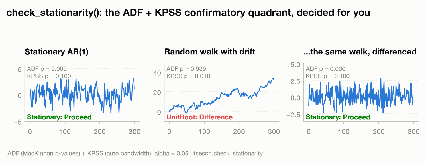
The figure shows the full loop on the gallery's synthetic data: a stationary AR(1) (both tests agree — proceed), a random walk with drift (both agree — difference), and the differenced walk (proceed again). The component tests are available standalone as tsecon.adf (with MacKinnon p-value response surfaces rather than sparse tables) and tsecon.kpss (automatic bandwidth); Chapter 4 of this guide dissects how they actually work, their deterministic-term cases, and their failure modes.
One distinction to file away now: a unit-root process (difference-stationary) is not the only way to trend. A trend-stationary series, \(Y_t = a + bt + u_t\) with \(u_t\) stationary, also rises forever — but its shocks are temporary and the right treatment is detrending (subtracting the fitted line), not differencing. The two look similar in levels yet imply opposite economics (recessions fully heal vs. leave permanent scars) and demand different surgery; check_stationarity's trend-aware variants and the KPSS "ct" regression option speak to this case, and the debate over which description fits GDP — reopened by Perron (1989), who showed a trend-stationary model with rare breaks can masquerade as a unit root — is still not fully settled.
The lag operator: the field's notation
Before going further, meet the notation the entire literature is written in. The lag operator \(L\) shifts a series back one period:
That looks like a triviality. Its power is that \(L\) behaves algebraically like a number — you can add, multiply, and form polynomials in it — which turns statements about dynamics into statements about polynomials. Three pieces of vocabulary built from it will recur in every later chapter:
The difference operator. \(\Delta = 1 - L\), so \(\Delta Y_t = Y_t - Y_{t-1}\): the period-over-period change. The seasonal difference is \(\Delta_s = 1 - L^s\), giving \(Y_t - Y_{t-s}\) — this quarter versus the same quarter last year when \(s = 4\).
Lag polynomials. The AR(1) rearranges to
and a general AR(p) is \(\phi(L)\,Y_t = \varepsilon_t\) with \(\phi(L) = 1 - \phi_1 L - \cdots - \phi_p L^p\). The dynamic properties of the process are encoded in the roots of the polynomial \(\phi(z) = 0\): the process is stationary when all roots lie outside the unit circle. Set \(\phi = 1\) in the AR(1) and the polynomial \((1 - L)\) has its root at 1 — literally a unit root, which is where the name you have been reading all chapter comes from. A unit root in \(\phi(L)\) means a factor of \((1-L)\) — that is, the process is something stationary that has been summed up, and \(\Delta\) is the operator that unwinds it.
Inversion. When \(|\phi| < 1\) the polynomial can be inverted like a geometric series, \((1 - \phi L)^{-1} = 1 + \phi L + \phi^2 L^2 + \cdots\), giving
the AR(1) is a weighted sum of all past shocks with geometrically fading weights. This two-way traffic between autoregressive form and moving-average form — made mechanical by lag-polynomial algebra — is the engine of Chapter 2, and its deep license is Wold's (1938) decomposition theorem: every weakly stationary process is a (possibly infinite) moving average of white noise. The atom really is universal.
Transformations: making data modelable
Raw economic data rarely arrives stationary, and the first practical modeling decision is which transformation to apply. Each addresses a specific pathology; applying the wrong one creates problems rather than solving them.
Logs fix level-dependent scale. GDP at $25 trillion fluctuates in dollar terms enormously more than GDP at $5 trillion did, because economies move in proportional terms. Taking \(\log Y_t\) converts equal percentage moves into equal absolute moves, stabilizing variance and turning exponential growth into a straight line. Rule of practice: any positive series spanning a large range (GDP, price indexes, stock levels, money aggregates) gets logged before anything else.
Differences remove unit roots. If \(Y_t\) is \(I(1)\), then \(\Delta Y_t\) is stationary and modelable — this is Difference, the recommendation check_stationarity printed for the random walk. Difference the log and you get both fixes at once:
the growth rate — the approximation is excellent for the small changes typical of quarterly data (within about 0.1 percentage point when growth is under 5%). This is why applied macro runs on log-differences: quarterly GDP growth, inflation as \(\Delta \log CPI_t\), stock returns as \(\Delta \log P_t\). Two conventions to keep straight when reading data releases: the same quarterly growth may be reported annualized (multiplied by 4, roughly — US convention) or as year-over-year (\(\log Y_t - \log Y_{t-4}\), a smoother but more lagging measure).
Box-Cox generalizes the choice between "log" and "don't log." Box and Cox (1964) defined the family
which nests no transformation (\(\lambda = 1\)), the log (\(\lambda = 0\)), and everything between — a square-root-like \(\lambda = 0.5\) often suits count-flavored data whose variance grows with the level but slower than proportionally. The parameter \(\lambda\) can be chosen automatically to stabilize variance, and tsecon.box_cox_lambda ships both standard routes: Guerrero's (1993) grouped coefficient-of-variation criterion (method="guerrero", the R forecast default) and the Box and Cox profile likelihood (method="mle"). The worked example at the end of this chapter runs it. Two practical warnings: the transform needs strictly positive data (zeros require a shift, applied honestly and documented), and forecasts made on the transformed scale must be back-transformed with a bias adjustment — naively inverting gives the forecast median, not the mean.
Choosing among them is a diagnosis, not a ritual. Variance growing with the level → log (or Box-Cox). Unit root → difference. Deterministic trend with stationary deviations → detrend instead. Often the answer is a pipeline: log, then difference, then model.
⚠ Common mistake: over-differencing. Differencing a series that was already stationary — or differencing when detrending was the right call — does not just waste a data point. It injects artificial negative autocorrelation (the ACF of an over-differenced series shows a telltale spike near \(-0.5\) at lag 1) and strictly destroys information, making forecasts worse. Differencing is medicine for a diagnosed unit root, not a vitamin taken for general health. Let
check_stationarity— ortsecon.ndiffs, the sequential differencing advisor demonstrated at the end of this chapter — prescribe the dose.
Frequency and seasonality: the vocabulary
A last block of vocabulary, because data documentation assumes you know it and the wrong word costs real money in misread releases.
The frequency of a series is its observation rate, conventionally counted per year: annual (1), quarterly (4), monthly (12), weekly (~52), daily (252 trading days or 365 calendar days), and up into the intraday realm econometricians call high-frequency. The period of a recurring pattern is how many observations it takes to repeat: 4 for a quarterly-data annual cycle, 12 for monthly.
Seasonality is the within-year pattern that recurs at a fixed, calendar-locked period: retail sales spike every December, construction slumps every winter, tax refunds land every spring. Distinguish it from a cycle, whose fluctuations recur at irregular intervals — the business cycle runs roughly 2 to 8 years but no fixed length, which is exactly why it needs the model-based extraction methods of the trend-cycle chapter rather than a calendar rule. Seasonality itself comes in two flavors that echo this chapter's central dichotomy: deterministic (a fixed December effect, removable with dummy variables) and stochastic (a seasonal pattern that itself drifts over the years — formally a seasonal unit root, removable only by seasonal differencing \(\Delta_s\)).
Most published macro series arrive seasonally adjusted (SA) — the statistical agency has already estimated and removed the seasonal component; the raw version is NSA (not seasonally adjusted). US data releases typically quote flows at a SAAR (seasonally adjusted annual rate): the quarterly figure scaled to a yearly pace. Related calendar effects — a month containing five weekends, the moving date of Easter or Lunar New Year — are removed in the same adjustment pipeline.
⚠ Common mistake: double-adjusting. Fitting seasonal dummies or seasonal differences to data that is already SA removes a component that is not there, distorting the dynamics that are (and residual traces of imperfect official adjustment are a known trap for automated model selectors). Equally classic in the other direction: comparing December NSA retail sales to November's and announcing a boom. Always check the SA/NSA flag before touching a series — it is the first line of the metadata for a reason.
The frontier
Everything above is settled science; here is where the settled part ends.
The unit-root question is less binary than this chapter made it. Near-unit-root processes (\(\phi = 0.98\), say) are, in finite samples, nearly indistinguishable from exact unit roots — Cochrane (1991) sharpened this into a near-observational-equivalence result: for any unit-root process there is a stationary one (and vice versa) that no test can tell apart at any given sample size. Modern practice therefore treats the ADF/KPSS verdict as a modeling decision rather than revealed truth, and the research frontier has moved toward procedures that hedge: the union-of-rejections strategies of Harvey, Leybourne, and Taylor combine tests across specifications, and inference methods robust to the \(I(0)/I(1)\) divide sidestep the pretest entirely. Structural breaks compound the problem — Perron (1989) showed one break can make a stationary series test as \(I(1)\) — which is why break-robust unit-root testing (Zivot-Andrews and successors) is a live subfield; the Zivot-Andrews test itself is a call, tsecon.zivot_andrews.
Between \(I(0)\) and \(I(1)\) lies a continuum. Fractionally integrated ("long memory") processes, introduced by Granger and Joyeux (1980) and Hosking (1981), have autocorrelations that decay hyperbolically rather than geometrically — too slow for ARMA, too fast for a unit root. Realized volatility in finance is the canonical example. Estimating the memory parameter \(d\) and distinguishing true long memory from spurious long memory caused by breaks (Qu's test) are active topics, and Python tooling is thin — neither statsmodels 0.15 nor arch 8.0 estimates \(d\) at all. tsecon ships the two standard estimators as tsecon.long_memory_d (Geweke-Porter-Hudak log-periodogram regression and Robinson's local Whittle), plus frac_diff/frac_integrate for the transform itself; the Shimotsu-Phillips exact-local-Whittle variant and Qu's break-versus-memory test are still open.
Stationarity itself is being relaxed. Locally stationary processes (Dahlhaus 1997) allow the DGP's parameters to drift smoothly, formalizing the intuition that the economy of 1960 and the economy of 2020 are not literally the same machine while preserving enough structure for inference. Tests for second-order stationarity (Priestley-Subba Rao; Nason's wavelet-based test) ask the data whether the constancy assumed all chapter actually holds.
On the library side, this chapter's scope sits inside Module 01. The module's flagship, the check_series() one-call diagnostic battery, is shipped: the codified unit-root decision logic with an evidence table rather than a bare verdict, ending in recommendations that route to concrete calls (see its model card). The rest of the unit-root family has landed alongside it: dfgls (Elliott-Rothenberg-Stock GLS detrending), ng_perron (the four M-tests with MAIC lag selection), and zivot_andrews (one endogenous break) are all callable, as are the ndiffs/nsdiffs differencing advisors and box_cox_lambda. Still on the roadmap: Lee-Strazicich two-break unit roots and the seasonal unit roots (HEGY and Canova-Hansen — a genuine dead zone in Python today). The honest open problems: no test resolves near-observational equivalence (only more data or more assumptions do); the multiple-testing problem in diagnostic batteries is usually ignored in practice (check_series shows the test families and the expected-false-alarm arithmetic rather than silently correcting); and the deterministic-terms choice in unit-root testing (constant? trend?) remains an under-acknowledged researcher degree of freedom.
Which method when
| Situation | Reach for | Because |
|---|---|---|
| First look at any new series | tsecon.acf (with tsecon.pacf) |
The memory profile — none / geometric decay / stuck near 1 — immediately narrows what the series can be |
| Deciding whether to difference | tsecon.check_stationarity |
Joint ADF+KPSS logic with opposite nulls beats either test alone; returns a recommendation plus the evidence |
| Need the components' detail (lags, deterministic terms) | tsecon.adf, tsecon.kpss directly |
Full control over regression case and lag/bandwidth choices |
| Checking whether residuals are white noise | tsecon.ljung_box |
Formal portmanteau test across many lags; the model-adequacy standard |
| Positive series whose swings grow with its level | np.log before modeling |
Converts proportional variation to additive; exponential growth to linear trend |
| Confirmed unit root | np.diff (on logs, for growth rates) |
Differencing removes the unit root; log-difference ≈ growth rate |
| Trend with stationary deviations around it | Detrend (regress on time), don't difference | Differencing a trend-stationary series over-differences and distorts dynamics |
| Neither log nor level obviously right | tsecon.box_cox_lambda (method="guerrero" or "mle") |
Nests both and everything between; data-driven λ |
| How many differences, decided by rule not by eye | tsecon.ndiffs (seasonal: tsecon.nsdiffs) |
The Hyndman-Khandakar sequential rule, with the test evidence at every order |
| ADF is inconclusive and the sample is short | tsecon.dfgls, tsecon.ng_perron |
GLS detrending buys power near the null; the M-tests fix ADF's size under a negative MA root |
| Unit-root verdict on a series with an obvious level shift | tsecon.zivot_andrews |
One endogenous break inside the test; plain ADF reads a broken mean as a unit root |
| Two trending levels look related | Stop — test for cointegration (later chapter) | Levels-on-levels regression of \(I(1)\) series is spurious by default |
| Seasonal pattern in NSA data | tsecon.seasonal_strength/tsecon.nsdiffs to decide, then tsecon.stl/tsecon.mstl or dummies |
Match the treatment to deterministic vs. stochastic seasonality |
What tsecon implements today
Available now in Python (everything this chapter ran):
tsecon.acf(y, nlags=20, adjusted=False)— sample ACF with Bartlett standard errors ("acf","bartlett_se")tsecon.pacf(y, nlags=20, method="yw")— partial autocorrelation (Yule-Walker or"ols")tsecon.check_stationarity(y, alpha=0.05)— the joint ADF+KPSS workflow: quadrant, recommendation, interpretation, and both tests' statisticstsecon.adf(y, regression="c", autolag="aic")— augmented Dickey-Fuller with MacKinnon p-value response surfacestsecon.kpss(y, regression="c", nlags=None)— KPSS with automatic (Hobijn-Franses-Ooms) bandwidthtsecon.ljung_box(y, nlags=10)— white-noise portmanteau test, Ljung-Box and Box-Pierce variantstsecon.check_series(data, seasonal_period=None, alpha=0.05)— the flagship one-call diagnostic battery: this chapter's tests (and chapter 2's) run in order, on the right scale, ending in recommendations that route to concrete calls — see the model cardtsecon.box_cox_lambda(y, method="guerrero"|"mle", bounds=..., period=2)— the variance-stabilizing λ, with the objective at the optimum and anat_boundflag; strictly positive data requiredtsecon.ndiffs(y, test="kpss"|"adf"|"pp", alpha=0.05, max_d=2)— the Hyndman-Khandakar sequential differencing advisor, returningdplus the per-order test evidence instepstsecon.nsdiffs(y, period, max_d=1)— the seasonal counterpart, theforecast::nsdiffs(test="seas")seasonal-strength rule over the shippedtsecon.stltsecon.dfgls(y, regression="c"|"ct")— DF-GLS (Elliott-Rothenberg-Stock 1996), matchingarch.unitroot.DFGLSto 1e-10tsecon.ng_perron(y, trend="c"|"ct")— the four Ng-Perron (2001) M-tests with MAIC lag selection; critical values only, because no published p-value surface existstsecon.zivot_andrews(y, regression="c"|"t"|"ct", trim=0.15)— unit root against stationarity around one endogenous break, matching statsmodels'zivot_andrews
Built in Rust awaiting bindings: nothing in this chapter's scope — the foundations layer is fully exposed to Python today.
The λ-and-differences pair from the transformations section, run end to end on a positive, exponentially growing series — the shape logs were invented for:
gdp = 1000.0 * np.exp(0.006 * np.arange(n) + 0.03 * walk)   # positive, proportional noise

bc = tsecon.box_cox_lambda(gdp, method="guerrero")   # automatic variance-stabilizing λ
print(round(bc["lambda"], 2))                        # -0.12 — essentially the log (λ = 0)

nd = tsecon.ndiffs(np.log(gdp))                      # how many differences to stationarity
print(nd["d"], nd["stop"])                           # 1 Stationary
Guerrero lands within a rounding error of \(\lambda = 0\), which is the data agreeing with the rule of practice this chapter gave you — log a positive series that spans a large range — and ndiffs then says the logged series needs exactly one difference, the log-difference growth rate. Both answers carry their evidence: bc["objective"]/bc["at_bound"] for the optimum, nd["steps"] for the KPSS statistic and p-value at every order tried.
Roadmap (Module 01 — Diagnostics, Exploration, Filters, and Seasonal Adjustment): Lee-Strazicich two-break unit roots, seasonal unit roots (HEGY, Canova-Hansen), and macro data utilities (growth rates, annualization, rebasing).
Further reading
- Yule (1926), "Why do we sometimes get nonsense-correlations between time-series?", Journal of the Royal Statistical Society — the founding document of the spurious-correlation problem, still startlingly readable.
- Slutsky (1927; English translation 1937, Econometrica), "The summation of random causes as the source of cyclic processes" — the discovery that accumulating pure noise manufactures apparent cycles; the random walk's deep lesson, a half-century early.
- Wold (1938), A Study in the Analysis of Stationary Time Series — the decomposition theorem: every stationary process is a moving average of white noise, the license for everything ARMA.
- Granger and Newbold (1974), "Spurious regressions in econometrics", Journal of Econometrics — the Monte Carlo bombshell: independent random walks reject the no-relationship null most of the time.
- Phillips (1986), "Understanding spurious regressions in econometrics", Journal of Econometrics — the asymptotic theory explaining why, showing the t-statistic diverges with sample size.
- Nelson and Plosser (1982), "Trends and random walks in macroeconomic time series", Journal of Monetary Economics — the empirical case that macro aggregates carry unit roots; reshaped macroeconomics and launched two decades of unit-root econometrics.
- Kwiatkowski, Phillips, Schmidt, and Shin (1992), "Testing the null hypothesis of stationarity against the alternative of a unit root", Journal of Econometrics — the stationarity-null complement that makes confirmatory testing possible.
- Box and Cox (1964), "An analysis of transformations", Journal of the Royal Statistical Society, Series B — the transformation family that frames log-vs-level as an estimable question.
- Box and Jenkins (1970), Time Series Analysis: Forecasting and Control — the book that turned the concepts of this chapter into a modeling workflow; its identify-estimate-diagnose loop is still the skeleton of applied practice.
- Hamilton (1994), Time Series Analysis — the field's encyclopedic graduate reference; rigorous treatments of everything this guide introduces, from the lag operator to unit-root asymptotics.
Next: Chapter 2 builds on these foundations to construct the ARMA family — the workhorse models for stationary series — and the Box-Jenkins workflow for choosing among them.