Chapter 12 — Machine Learning for Time Series
Part of The tsecon Guide to Time Series Econometrics. Chapters mirror the library's modules; code runs against the current Python API unless marked otherwise.
Prerequisites: OLS regression, the bias-variance idea, and the forecasting-evaluation toolkit (MASE, the Diebold-Mariano test) from the previous chapters.
You will learn:
- Why the standard machine-learning playbook — random K-fold cross-validation — produces fraudulent accuracy numbers on serial data, and how purging, embargoes, and rolling-origin evaluation fix it
- How ridge, LASSO, and elastic net trade a little bias for a lot of variance, and how they connect to the Bayesian shrinkage of Chapter 10
- Why factor models were machine learning before the name existed, and why they remain the benchmark to beat
- What the honest evidence says about trees, boosting, neural networks, and foundation models in macroeconomic forecasting
- Why you should almost never believe the story told by which variables LASSO selects
The idea
Suppose you are asked to forecast US inflation twelve months out. You have the FRED-MD panel: about 130 monthly macroeconomic series — production, employment, housing starts, interest rates, money aggregates, exchange rates — going back to 1959. Classical practice says: pick a small model, maybe an AR(4) or a Phillips-curve regression, and ignore the other 125 series. That feels wasteful. Machine learning says: use everything, and let the algorithm decide what matters.
That instinct is often right, and this chapter is about making it work. But the first thing that breaks when you point ML at economic data is not the model — it is the scorecard. The standard ML recipe for measuring accuracy shuffles the data into random chunks, trains on most of them, and tests on the rest. With cross-sectional data (say, house prices) this is fine, because the observations do not know about each other. A time series is different: it remembers. This month's industrial production is nearly a copy of last month's. If March 2008 is in your test set while February and April 2008 sit in the training set, the model has effectively been shown the answer before the exam. It will score brilliantly and forecast terribly.
Picture two report cards for the same model. One is graded by a teacher who shuffles the exam questions in among the practice problems — the student has seen the neighbors of every question. The other is graded the only way the real world grades a forecaster: stand at a date, use only what was known then, predict forward, move the date, repeat. The first report card is flattering fiction. The second is the truth. Everything else in this chapter — penalized regressions, factor models, forests, neural networks — only means something once you insist on the second report card. So we start there, with the fraud, before we get to the models.
Leakage comes first
Leakage is any path by which information from the evaluation period reaches the model during training. It is the cardinal sin of applied ML, and time series data makes it shockingly easy to commit. A practitioner cares because leakage does not make results look slightly better — it routinely turns a worthless model into an apparent star, and it has contaminated a nontrivial share of published "ML beats econometrics" claims.
The mechanics. Cross-validation (CV) estimates out-of-sample accuracy by splitting the data into K folds (chunks), training on K−1 of them, and testing on the held-out fold, rotating until every fold has been the test set. Its validity rests on the training and test sets being informationally separated. Serial dependence destroys that separation in two ways:
- Neighbor leakage. With random folds, almost every test observation is temporally sandwiched between training observations that are highly correlated with it. The model can interpolate rather than forecast.
- Overlap leakage. When you forecast h steps ahead, even a correctly specified model has serially correlated errors. Write the series in terms of its shocks (the Wold form of Chapter 2): the h-step-ahead forecast error is
where \(\varepsilon_t\) are the one-step shocks and \(\psi_j\) the moving-average weights. Two forecast errors dated less than h periods apart share shocks — h-step errors follow an MA(h−1) process. A training row whose target window overlaps a test row's target window is made of the same randomness the test asks you to predict.
Three repairs, in increasing order of caution:
- Rolling-origin evaluation (also called pseudo-out-of-sample, POOS): stand at origin \(t\), fit using only data observable at \(t\), forecast \(t+h\), advance the origin, repeat. This is the gold standard because it simulates real forecasting exactly, including re-estimation.
- Purging: if you must use fold-based CV (it is K times cheaper than rolling origin when tuning many hyperparameters), make folds contiguous blocks, never shuffled, and delete from the training set any row whose target window overlaps the test block — every row within h−1 of it.
- Embargo: additionally drop a buffer of rows immediately after the test block. This guards against slower leakage channels — features built from smoothed or slow-moving transforms that carry test-period information forward (López de Prado 2018 introduced the purge/embargo terminology in the finance-ML setting). The embargo should scale with the forecast horizon.
Here is the split logic, in plain numpy — this is the pattern every honest backtest in this chapter uses:
import numpy as np

def rolling_origin_splits(n_rows, h, first_origin):
    """Row i's features end at time i; its target is at time i + h.
    Train only on rows whose targets are already observed at the origin."""
    for origin in range(first_origin, n_rows):
        yield np.arange(0, origin - h + 1), origin

def purged_kfold_splits(n_rows, n_folds, h, embargo=0):
    """Contiguous folds. Purge training rows within h-1 of the test block
    (their target windows overlap it); embargo a further buffer after it."""
    all_rows = np.arange(n_rows)
    for fold in np.array_split(all_rows, n_folds):
        lo, hi = fold[0], fold[-1]
        keep = (all_rows <= lo - h) | (all_rows >= hi + h + embargo)
        yield all_rows[keep], fold
One honest nuance, because blanket rules breed cargo cults: Bergmeir, Hyndman & Koo (2018) prove that ordinary K-fold CV is valid for purely autoregressive models with uncorrelated errors. The intuition: if the model's inputs are lags of the series and the errors are genuinely unpredictable noise, having temporal neighbors in the training set tells the model nothing about the test-period noise. The trouble is that the conditions are fragile — one-step horizon, correctly specified lag structure, no external features, no memorizing model. The moment you add a smoothed feature, a trend index, a multi-step horizon, or a flexible learner, the theorem no longer protects you. Rolling origin is never wrong; K-fold is sometimes right. Price that asymmetry accordingly.
You have already seen this movie in a different theater. In Chapter 1's bootstrap discussion, iid resampling of an autocorrelated series destroyed the dependence structure and produced confidence intervals roughly three times too narrow:
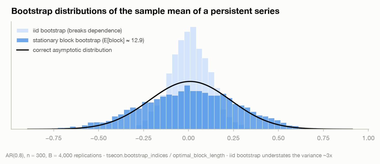
Random K-fold CV is the same pathology wearing a different hat: an iid assumption applied to dependent data, quietly understating uncertainty — here, understating forecast error.
⚠ Common mistake. Standardizing (or differencing, detrending, imputing, or selecting features) on the full sample before splitting. The test data's mean and variance leak into every training fold through the scaler. Every transform must be fit on training data only, inside each split — the tsecon roadmap's pipeline protocol enforces this mechanically, and property-tests it: perturbing data after a fold boundary must not change any fitted transform.
A teachable disaster: one model, two backtests
Nothing makes the point like watching the same model get two different grades. The demo below builds a series that is, by construction, unforecastable beyond a drift-adjusted "no-change" guess: a random walk with drift. The "ML model" is a 3-nearest-neighbor regression — for each new feature vector, find the 3 most similar training rows and average their targets. The feature set is four lags plus a trend index (the row number), the kind of harmless-looking calendar feature that ML pipelines add reflexively. Everything runs today:
import numpy as np
import tsecon

# --- A series nothing should beat: a random walk with drift ---------------
rng = np.random.default_rng(42)
n, p, h = 500, 4, 8                       # sample size, lags, forecast horizon
y = 0.2 * np.arange(n) + np.cumsum(rng.standard_normal(n))

# Supervised design: row i holds lags (y_t, ..., y_{t-3}) plus a trend index;
# its target is y_{t+8}. The trend index looks harmless. It is not.
rows = np.arange(p - 1, n - h)
X = np.column_stack([y[rows - j] for j in range(p)] + [rows.astype(float)])
target = y[rows + h]

def knn(X_tr, y_tr, x_new, k=3):          # the "ML model": 3-nearest-neighbor
    d = np.abs(X_tr - x_new).sum(axis=1)
    return y_tr[np.argsort(d)[:k]].mean()

# --- Backtest 1: the LEAKY protocol ---------------------------------------
# Sin 1: standardize features on the FULL sample (test data leaks into scaling).
# Sin 2: random K-fold — test rows sit surrounded by their temporal neighbors.
Xz = (X - X.mean(0)) / X.std(0)
perm = rng.permutation(len(rows))
leaky_pred = np.empty(len(rows))
for fold in np.array_split(perm, 5):
    train = np.setdiff1d(perm, fold)
    for i in fold:
        leaky_pred[i] = knn(Xz[train], target[train], Xz[i])

# --- Backtest 2: the HONEST protocol (rolling origin + purge) -------------
start = 250                                # first forecast origin
oos = np.arange(start, len(rows))
honest_pred, naive_pred = np.empty(len(oos)), np.empty(len(oos))
for j, i in enumerate(oos):
    train = np.arange(0, i - h + 1)        # purge: keep rows whose target is
    mu, sd = X[train].mean(0), X[train].std(0)   # already observed at the origin
    honest_pred[j] = knn((X[train] - mu) / sd, target[train], (X[i] - mu) / sd)
    drift = np.diff(y[: rows[i] + 1]).mean()     # benchmark: drift-adjusted
    naive_pred[j] = y[rows[i]] + h * drift       # no-change forecast

# --- Scoring: same evaluation rows, same metrics --------------------------
actual, insample = target[oos], y[: rows[start] + 1]
for name, pred in [("leaky", leaky_pred[oos]), ("honest", honest_pred),
                   ("naive", naive_pred)]:
    a = tsecon.accuracy(actual, pred, insample=insample)
    print(f"{name:7s} RMSE {a['rmse']:5.2f}   MASE {a['mase']:5.2f}")

dm = tsecon.dm_test(actual - naive_pred, actual - honest_pred, h=h)
print(f"DM (naive vs model, honest errors): stat {dm['hln_stat']:.2f}, "
      f"p = {dm['p_value']:.3f}")
The output:
leaky   RMSE  1.19   MASE  1.24
honest  RMSE  4.38   MASE  4.49
naive   RMSE  2.99   MASE  3.12
DM (naive vs model, honest errors): stat -2.34, p = 0.020
Read the disaster carefully, because both halves teach something:
- The leaky backtest says the model is a triumph: RMSE 1.19 against the no-change benchmark's 2.99 — "our ML model beats the random walk by 60%." The mechanism is memorization: after full-sample z-scoring, the trend index makes each row's nearest neighbors its immediate temporal neighbors, and random folds guarantee those neighbors are in the training set. Their targets share almost all their shocks with the test target (the MA(h−1) overlap made flesh). The model is not forecasting; it is looking up the answer key.
- The honest backtest says the model is a liability: RMSE 4.38 — 47% worse than no-change, and the Diebold-Mariano test (from the forecasting-evaluation chapter; here
e1is the benchmark, so a negative statistic favors it) says the deficit is statistically real (p = 0.02). The same trend feature that powered the illusion now sabotages genuine forecasts: at a real out-of-sample origin, the current trend value lies outside everything in the training set, so nearest-neighbor lookup grabs stale rows and systematically under-predicts. Flexible learners interpolate beautifully and extrapolate badly.
The gap between the two report cards — MASE 1.24 versus 4.49 for the same model on the same data — is the entire argument of this section. The leaky number is the one that would have gone in the paper.
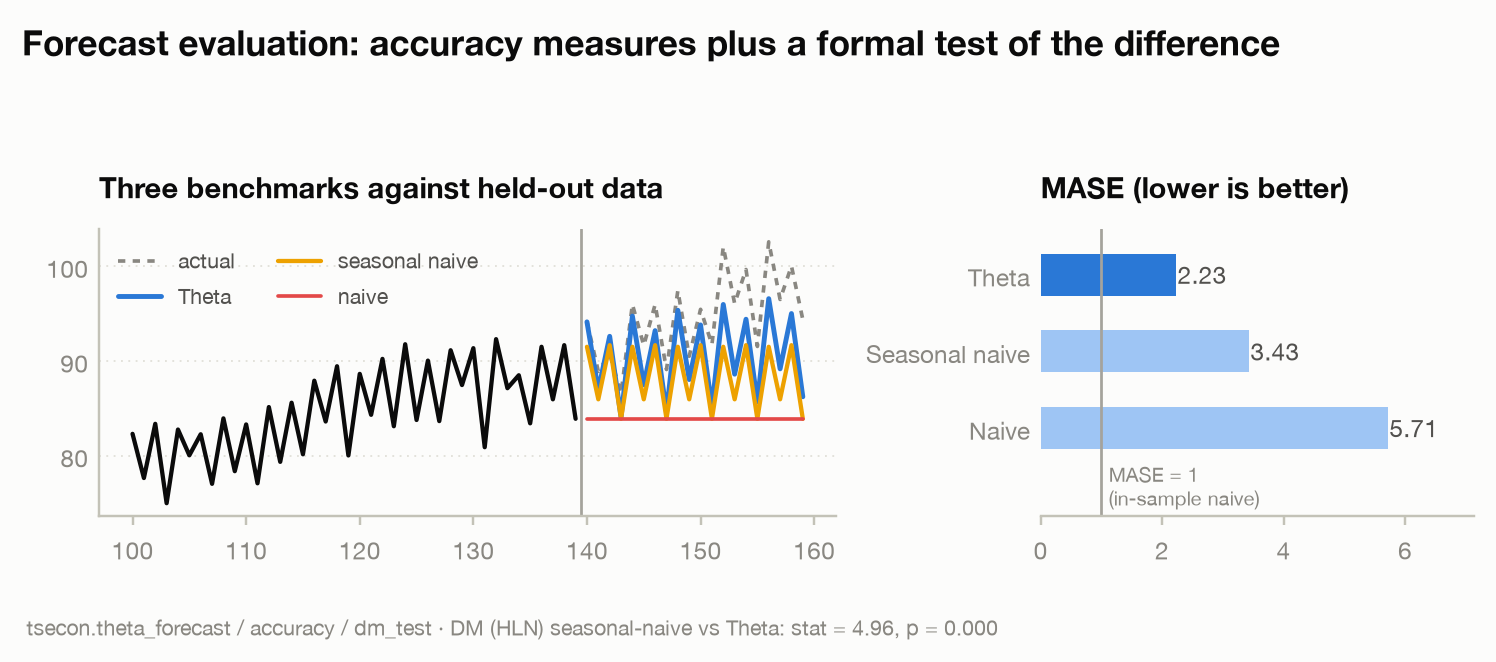
The scoring machinery (tsecon.accuracy, tsecon.dm_test) is the same discipline layer used everywhere in the library — never report a forecast without a benchmark, never claim superiority without a test:
⚠ Common mistake. Fixing the leak in evaluation but not in tuning. If you select hyperparameters (a penalty weight, tree depth, k) by leaky CV and then report performance from an honest holdout, the damage is smaller but still real: you have optimized the model for interpolation, not forecasting, and you have used the holdout once per tuning decision. Tune and evaluate with dependence-aware splits, and keep a final untouched window if the model will face real money or real policy.
Shrinkage with a frequentist face
Now the models. The workhorse of data-rich forecasting is not deep learning — it is penalized linear regression. A practitioner cares because the typical macro problem has dozens-to-hundreds of candidate predictors (and each contributes several lags) against a few hundred observations. OLS in that regime is unbiased and useless: the variance of the coefficient estimates overwhelms any signal. Shrinkage — deliberately biasing coefficients toward zero to slash their variance — is the classic bias-variance trade, and it usually wins.
The unified estimator is the elastic net (Zou & Hastie 2005), which contains ridge and LASSO as endpoints:
where \(\lambda \ge 0\) sets the overall penalty strength, and \(\alpha \in [0,1]\) mixes the two penalty geometries. \(\alpha = 0\) is ridge (Hoerl & Kennard 1970): the squared L2 penalty shrinks every coefficient smoothly toward zero but never exactly to zero — right for dense problems where many predictors carry a little signal. \(\alpha = 1\) is the LASSO (Tibshirani 1996): the absolute-value L1 penalty has a kink at zero that sets many coefficients exactly to zero, performing variable selection and estimation in one step — right for sparse problems where a few predictors carry most of the signal. Intermediate \(\alpha\) matters for time series because lags of the same variable are highly collinear, and pure LASSO arbitrarily keeps one of two correlated lags while dropping the other; the ridge component stabilizes that choice. The adaptive LASSO (Zou 2006) reweights the penalty by first-stage estimates and is the theoretically preferred variant under dependence (Medeiros & Mendes 2016).
This should feel familiar from Chapter 10. Ridge is exactly the posterior mean of a regression with a Gaussian prior centered at zero; the LASSO solution is the posterior mode under a Laplace prior. Shrinkage is one idea wearing two costumes — the Minnesota prior shrinking a VAR toward a random walk and a ridge penalty shrinking a forecasting regression toward zero are the same move, differing in what they shrink toward and how they choose the strength. The frequentist face tunes \(\lambda\) by cross-validation or information criteria; the Bayesian face integrates over it.
Ridge is a two-line closed form, so the demo below writes it out in numpy — the point is to watch rolling-origin tuning pick \(\lambda\), not to hide the estimator. Truth here is an AR(2); the design offers 24 lags against roughly 100 usable observations:
import numpy as np

rng = np.random.default_rng(7)
n, p = 120, 24                        # 24 candidate lags, ~100 usable rows
eps = rng.standard_normal(n)
y = np.zeros(n)
for t in range(2, n):                 # truth: AR(2) — only two lags matter
    y[t] = 0.5 * y[t-1] - 0.3 * y[t-2] + eps[t]

rows = np.arange(p, n - 1)
X = np.column_stack([y[rows - j] for j in range(p)])
target = y[rows + 1]

def ridge(X_tr, z, lam):              # closed form: (X'X + lam*I)^{-1} X'z
    return np.linalg.solve(X_tr.T @ X_tr + lam * np.eye(X_tr.shape[1]),
                           X_tr.T @ z)

def honest_rmse(lam, start=60):       # rolling origin, one step, purged
    e = [target[i] - X[i] @ ridge(X[:i], target[:i], lam)
         for i in range(start, len(rows))]
    return np.sqrt(np.mean(np.square(e)))

grid = np.geomspace(0.1, 1000.0, 25)
lam_star = grid[np.argmin([honest_rmse(lam) for lam in grid])]
print(f"lambda* = {lam_star:.0f}")                       # heavy shrinkage: 464
print(f"OLS  {honest_rmse(1e-8):.3f}")                   # 1.107
print(f"ridge {honest_rmse(lam_star):.3f}")              # 0.960
Unpenalized OLS pays a 15% RMSE premium for estimating 22 coefficients that are truly zero; tuned ridge gets within a whisker of the noise floor (the innovation standard deviation is 1.0). That is the whole shrinkage story in three lines of output.
You do not have to keep the hand-rolled solver. tsecon.ridge(X, y, alpha=lam_star) returns the same coefficient vector — it is the same closed form, matching the ridge above to \(7 \times 10^{-17}\) on this design, against scikit-learn's Ridge objective (add your own intercept column if you want one). The plain tsecon.lasso is its L1 twin. Swap it in and the loop above is unchanged; the folds are the part that has to stay honest, not the linear algebra.
Two structured extensions matter for time series designs. The group LASSO (Yuan & Lin 2006) penalizes coefficients in pre-declared groups by \(\lambda \sum_g \sqrt{p_g}\, \lVert \beta_g \rVert_2\), so a group — naturally, all lags of one variable — enters or leaves the model as a unit; selection happens at the economic level ("does oil matter?") rather than the lag level ("does the seventh lag of oil matter?"). The sparse-group LASSO (Simon, Friedman, Hastie & Tibshirani 2013) mixes in a within-group L1 term so a selected variable can still use only a few of its lags — it is also the engine under the nowcasting chapter's MIDAS regressions. For tuning, information criteria are often preferable to CV in time series (faster, no splitting subtleties): for the LASSO the degrees of freedom equal the number of nonzero coefficients exactly (Zou, Hastie & Tibshirani 2007), making BIC well-defined; when the predictor count outruns the sample, use the extended BIC (Chen & Chen 2008) or BIC will overselect catastrophically.
The path solver has since landed as tsecon.lasso_path (taught in full below); the elastic-net blend is the same call with l1_ratio < 1, and the information criteria come back with it. When you already know the penalty and want a single fit rather than the whole path, tsecon.elastic_net(x, y, alpha, l1_ratio=0.5) solves that one scikit-learn-convention objective directly (see the machine-learning model card). On the 24-lag AR(2) design from the ridge example above:
path = tsecon.lasso_path(X, target)                    # glmnet-convention LASSO path
enet = tsecon.lasso_path(X, target, l1_ratio=0.5)      # l1_ratio<1 blends in the ridge penalty
print(f"LASSO path: {len(path['lambdas'])} lambdas; "
      f"BIC picks df={path['df'][path['bic_best']]}, AIC picks df={path['df'][path['aic_best']]}")
print(f"elastic net (l1_ratio=0.5): BIC picks df={enet['df'][enet['bic_best']]}, "
      f"AIC picks df={enet['df'][enet['aic_best']]}")
LASSO path: 100 lambdas; BIC picks df=1, AIC picks df=8
elastic net (l1_ratio=0.5): BIC picks df=1, AIC picks df=9
The grouped variant — where all lags of one variable enter or leave together — ships as tsecon.group_lasso (0.8.0): one integer group label per column, a penalty alpha on the same \(1/2n\) scale as lasso, and l1_ratio > 0 to mix in the sparse-group term. Every fit returns its own subgradient KKT residual (kkt_violation), so converged is a certificate for this convex problem rather than an iteration count.
groups = np.arange(X.shape[1]) // 4                       # four consecutive lags share a label
grp = tsecon.group_lasso(X, target, groups, alpha=0.05)   # a variable enters/leaves as a unit
print("active groups:", grp["active_groups"], " KKT residual:", f"{grp['kkt_violation']:.1e}")
⚠ Common mistake. Reporting ordinary OLS standard errors on coefficients after any selection step. Selection is a data-dependent event; conditioning on it invalidates the usual distribution theory, and the resulting "t-statistics" are fiction. Refitting OLS on the selected support (post-LASSO, Belloni & Chernozhukov 2013) de-biases the point estimates but does not rescue the standard errors — for honest inference you need the desparsified LASSO or post-double-selection, both below. A second, quieter trap: penalized objectives differ across software in loss scaling (the \(1/2n\) above is the glmnet convention) and standardization defaults, so the same \(\lambda\) means different things in different packages. tsecon matches glmnet's conventions exactly so published \(\lambda\) values transfer.
Factor models: ML before it was cool
Dimension reduction by principal components was solving the "wide data" problem in economics two decades before the phrase "machine learning" entered the field's vocabulary. A practitioner cares because the diffusion index approach of Stock & Watson (2002, JASA; 2002, JBES) remains, on the evidence, roughly tied with penalized regression as the best simple thing you can do with a large macro panel — and it is the benchmark every ML paper must beat.
The model: a large standardized panel \(X_t\) (N series) is driven by a small number r of common factors \(F_t\),
where \(\Lambda\) (N × r) holds the loadings — how much each series responds to each factor — and \(e_t\) is series-specific noise. Estimate \(\hat F_t\) by principal components (the r directions capturing the most panel variance), then forecast with a small regression that any econometrician would recognize:
with \(\beta(L)\), \(\gamma(L)\) short lag polynomials. The factors compress 130 series into a handful of estimated indexes — empirically, a "real activity" factor, a "prices" factor, an "interest-rate spread" factor — and the forecasting equation stays low-dimensional, stable, and interpretable. The number of factors is chosen by the Bai & Ng (2002) information criteria; McCracken & Ng (2016) maintain the FRED-MD panel precisely so this literature has a common testbed. Refinements push the compression toward the forecast target rather than the panel's own variance: targeted predictors (Bai & Ng 2008) screen the panel for series relevant to \(y\) before extracting factors, and the three-pass regression filter (Kelly & Pruitt 2015) extracts factors supervised by the target directly. Factors also plug into structural work — the FAVAR of Bernanke, Boivin & Eliasz (2005) puts \(\hat F_t\) inside a VAR from Chapter 4.
Where does the ML framing earn its keep? Factor models are unsupervised learning — PCA is the textbook first example — followed by a supervised readout. Thinking of them that way clarifies both their power (they exploit the panel's pervasive comovement, exactly the structure that defeats sparse methods, as the next section explains) and their obligations (the entire pipeline, standardization and factor extraction included, must sit inside the honest backtest loop).
The PCA factor extraction has landed as tsecon.factor_model — principal-component factors with the Bai-Ng (2002) count built in. Here a 60-series panel is driven by three persistent common factors; the estimator recovers the count, and the factors forecast a factor-driven target better than its own past does:
import numpy as np, tsecon

# A large panel driven by a few persistent common factors (the Stock-Watson setup):
#   X_t = Λ F_t + e_t,  the factors following an AR(1) so they carry forecastable signal.
rng = np.random.default_rng(0)
T, N, r = 240, 60, 3
F = np.zeros((T, r))
for t in range(1, T):
    F[t] = 0.9 * F[t-1] + rng.standard_normal(r)          # persistent common factors
loadings = rng.standard_normal((N, r))
panel = F @ loadings.T + rng.standard_normal((T, N))

sel   = tsecon.factor_model(panel, kmax=8)                # Bai-Ng (2002) chooses the count
r_hat = sel["icp2"]
Fhat  = np.array(tsecon.factor_model(panel, n_factors=r_hat, kmax=8)["factors"])
print(f"Bai-Ng ICp2 selects {r_hat} factors (truth {r}); ICp1={sel['icp1']}, ER={sel['er']}")

# Supervised readout: forecast a factor-driven target h steps out from [const, F_t, y_t].
y, h = F @ np.array([1.0, -0.6, 0.4]) + 0.5 * rng.standard_normal(T), 4
def r2(cols):
    Xr = np.column_stack([np.ones(T - h)] + cols)
    p  = np.array(tsecon.ols(y[h:], Xr)["params"])
    return 1.0 - np.sum((y[h:] - Xr @ p) ** 2) / np.sum((y[h:] - y[h:].mean()) ** 2)
print(f"factor readout R^2 (h={h}) : {r2([Fhat[:-h], y[:-h]]):.3f}")
print(f"AR(1) benchmark  R^2 (h={h}) : {r2([y[:-h]]):.3f}")
Bai-Ng ICp2 selects 3 factors (truth 3); ICp1=3, ER=3
factor readout R^2 (h=4) : 0.184
AR(1) benchmark  R^2 (h=4) : 0.150
The factors carry predictive signal the target's own lag does not — the diffusion-index bet in miniature. A one-call factor_forecast facade (the supervised readout with automatic lag selection) is still on the roadmap; the lines above are all it would wrap.
⚠ Common mistake. Estimating factors once on the full sample and then "backtesting" the forecasting regression on subsamples. The factor estimates at date t now contain information from the entire future of the panel — leakage again, wearing a third hat. In a proper pseudo-out-of-sample exercise the factors are re-extracted at every origin from data observable at that origin. The difference is not academic: full-sample factors are visibly smoother and can flip the sign of apparent forecast gains.
Trees and boosting: when nonlinearity pays
Everything so far is linear. Regression trees partition the feature space by recursive binary splits ("is unemployment above 6%? is the yield-curve slope negative?") and predict a constant in each cell; a random forest (Breiman 2001) averages hundreds of trees, each grown on a resampled version of the data with random feature subsets, trading the tree's interpretability for dramatically lower variance. Gradient boosting builds an additive model by fitting each new tree to the residuals of the ensemble so far. These are the strongest off-the-shelf nonlinear learners in tabular ML. Do they help in macro?
The honest answer: sometimes, measurably, and we roughly know when. Medeiros, Vasconcelos, Veiga & Zilberman (2021) ran the definitive US inflation horse race on FRED-MD data and found random forests delivering RMSE gains of the order of 10–30% over benchmarks, including through the Great Recession. Goulet Coulombe, Leroux, Stevanovic & Surprenant (2022) dissected why across a broad set of targets: the gains come specifically from nonlinearity — regime-dependent predictive relationships, interactions, thresholds — and concentrate at longer horizons and in turbulent periods; the resampling and the feature-subsetting are supporting cast. The flip side is equally well documented: for smooth, persistent aggregates in short samples — most quarterly GDP-type problems — trees rarely beat a well-tuned ridge or factor model, and their step-function forecasts extrapolate trends poorly (recall the disaster demo: flexible learners interpolate, they do not extrapolate). If your prior is "linear with modest noise," shrinkage wins; if your prior is "the Phillips curve has a kink somewhere," forests can find it without being told where.
For econometricians, componentwise L2 boosting (Bühlmann & Yu 2003; applied to recessions by Ng 2014) deserves a special mention: each boosting step fits a single predictor-lag by least squares and adds a small fraction of it to the model. Read sequentially, it is an automated ARDL-building procedure — a variable selector that econometricians can audit line by line — and it is deterministic and cheap; it ships as tsecon.boosting, with Bühlmann's (2006) corrected-AIC rule choosing the stopping step. Simpler still, bagging a pretest rule (estimate, keep what is significant, average over bootstrap replicates — Inoue & Kilian 2008) captures much of the ensemble benefit with none of the machinery, and is a good pedagogical bridge from OLS to ensembles.
Two dependence-specific cautions govern all tree methods on time series. First, the resampling inside a forest assumes exchangeable observations; on serial data it has to draw blocks, not rows. Second — see the mistake box. Both ship natively since 0.8.0: tsecon.regression_tree is CART with scikit-learn's split conventions (golden-pinned to DecisionTreeRegressor), and tsecon.random_forest grows those trees on iid, moving-block or stationary row resamples (bootstrap="block" / "stationary" with a block_length), returning out-of-bag predictions, Meinshausen quantile forests (quantiles=), and impurity or grouped block-permutation importance — the time-series-aware pieces the module design asked for. Gradient-boosted trees (XGBoost, LightGBM) stay wrapped behind optional adapters rather than reimplemented. A third-party learner still slots into the same discipline: tsecon.cv_splits for the folds, tsecon.bootstrap_indices / tsecon.optimal_block_length for block resampling, and tsecon.backtest, which takes a plain Python callable as the forecaster.
⚠ Common mistake. Trusting a random forest's out-of-bag (OOB) error — the built-in accuracy estimate computed from trees that did not see each observation — as a forecast-accuracy measure. OOB is a random K-fold in disguise: the observations a tree did not see are temporal neighbors of the ones it did. Under autocorrelation OOB error is systematically optimistic. Always grade forests the same way as everything else: rolling-origin pseudo-out-of-sample metrics.
The sparsity illusion
The LASSO's great seduction is the story it tells: "of your 130 predictors, these seven matter." Before you build a narrative on that, read Giannone, Lenza & Primiceri (2021) — this section is the guide's version of required reading.
Their question is whether economic prediction problems are actually sparse (few big coefficients, rest zero — LASSO's home turf) or dense (many small coefficients — ridge's home turf). Rather than assuming an answer, they estimate it: a spike-and-slab regression (Chapter 10 machinery) in which the probability of inclusion \(q\) is itself an unknown parameter with a prior,
so the data can express a posterior belief about sparsity itself. Across six canonical economic prediction problems — macro forecasting with large panels among them — the posterior on \(q\) piles up away from zero: the data favor dense models. Worse for the storyteller, even when a sparse model predicts well, the posterior over which predictors to include is spread across many near-equivalent subsets. The apparent sparsity of a LASSO fit is largely an artifact of the penalty, not a discovery about the economy: collinear predictors (and macro panels are pervasively collinear, precisely because of the factor structure of the previous section) offer many equally good sparse representations, and the L1 kink picks one arbitrarily. Change the sample by a year and the selected set reshuffles while the forecasts barely move.
Practical consequences, in order of importance. First, expect ridge-type dense shrinkage and factor models to forecast at least as well as the LASSO on typical macro panels — the horse-race evidence (Smeekes & Wijler 2018; Medeiros et al. 2021) generally agrees. Second, when you do want sparsity under a factor structure, remove the common factors first and run selection on the idiosyncratic remainders — FarmSelect (Fan, Ke & Wang 2020) — or the factors will masquerade as whichever individual series the penalty happens to like. Third, and always: selection is a modeling convenience, not a causal finding.
⚠ Common mistake. Publishing the list of LASSO-selected variables with economic interpretation attached ("credit spreads drive inflation; money growth does not"). The selection event is unstable across samples, tuning choices, and collinear substitutes. If the identity of the predictors is the scientific question, you need the inference tools of the next section and the frontier — not a penalty's arbitrary tiebreak.
Causal machine learning with dependent data
Everything above chases predictive accuracy. Much of econometrics instead wants one number with a confidence interval: the effect of a policy variable \(d_t\) on an outcome \(y_t\), with many controls \(x_t\) whose functional form you would rather not specify. Double/debiased machine learning (DML) (Chernozhukov, Chetverikov, Demirer, Duflo, Hansen, Newey & Robins 2018) is the framework that lets flexible ML estimate the nuisance pieces while preserving valid inference on the parameter you care about. In the partially linear model
\(\theta\) is the target and \(g\), \(m\) are unknown nuisance functions. Two ideas make it work. Neyman orthogonality: estimate \(\theta\) from residualized quantities — regress \(y - \hat g(x)\) on \(d - \hat m(x)\) — so that first-order errors in \(\hat g\) and \(\hat m\) do not transmit to \(\hat\theta\) (this is Frisch-Waugh-Lovell wearing ML clothes). Cross-fitting: fit the nuisances on one part of the sample and form residuals on another, swapping roles, so the ML models' overfitting does not correlate with the errors they are cleaning. A simpler cousin for linear nuisances is post-double-selection (Belloni, Chernozhukov & Hansen 2014): run LASSO of \(y\) on controls, LASSO of \(d\) on controls, take the union of selected supports, and run OLS of \(y\) on \(d\) plus that union — never penalizing \(d\) itself.
With time series data, both ideas need repair, and this is where the chapter's opening theme returns with force. Cross-fitting's sample splits are random partitions — exactly the leaky construction of the disaster demo. Under serial dependence the folds must be contiguous blocks separated by embargo buffers scaled to the dependence horizon, or the nuisance fits leak test-period shocks and \(\hat\theta\)'s distribution theory quietly fails. And the variance of the orthogonal score inherits the serial correlation of \(u_t\) and \(v_t\), so the standard error must come from a HAC/long-run variance estimator (Chapter 3's tsecon.long_run_variance machinery, with all its bandwidth caveats), not the iid sample variance. Both repairs are engineering-grade in the library's design; the honest caveat is that the formal theory for DML under general dependence is still an active research area, so treat time-series DML output as carefully as you would any frontier method. For PDS with time-series controls (lags, deterministic terms), the same HAC discipline applies to the final OLS step.
⚠ Common mistake. Running an off-the-shelf DML package with its iid defaults — random cross-fitting folds and iid score variances — on time series or panel data with serial dependence. Nothing errors out; you simply get confidence intervals that are too narrow and folds that leak. Check what the software assumes before believing the second decimal of a standard error.
Neural forecasters and foundation models
Neural networks enter macro forecasting in three tiers, and the evidence deserves to be read tier by tier.
Small feedforward networks — one or two hidden layers on lagged inputs — are the "NN" line in the serious horse races (Medeiros et al. 2021; Goulet Coulombe et al. 2022). Verdict: competitive but rarely dominant; they capture the same nonlinearity premium as forests, at the cost of fussier optimization. Because training is nondeterministic (random initialization, floating-point reduction order across threads), respectable practice averages an ensemble over ~10 seeds and promises statistical, not bitwise, reproducibility. This is the one neural model the module design puts in the core rather than behind an adapter, and it ships as tsecon.mlp_regression (0.8.0): scikit-learn's exact objective, Adam or L-BFGS, early stopping on a temporal validation split, a seed ensemble (n_seeds) averaged into the forecast, and a scaler fitted on the training rows only. tsecon.echo_state_network adds reservoir computing at contrib grade. Anything heavier, wrap your own and grade it through tsecon.backtest.
Specialized deep forecasters — N-BEATS, N-HiTS, DeepAR, the Temporal Fusion Transformer — won fame on large panels of related series (retail demand, electricity, the M4/M5 competitions). Their sweet spot is cross-learning: thousands of related series sharing one model. Macro's typical regime — one target, a few hundred quarterly observations — is close to their worst case, and they seldom beat well-tuned classical benchmarks there.
Foundation models — Chronos (Ansari et al. 2024), TimesFM (Das et al. 2024), Moirai (Woo et al. 2024), Lag-Llama (Rasul et al. 2024), TimeGPT (Garza et al. 2023) — are pretrained on enormous corpora of time series and forecast new series zero-shot, no training required. The benchmark numbers are genuinely impressive, and for a practitioner with thousands of heterogeneous series and no time to model each one, they are a real option. For econometric use, three honest concerns temper the enthusiasm. Contamination: the pretraining corpora plausibly contain the very series (FRED, M-competition data) on which the models are evaluated, so a zero-shot "win" may be a memory. Small-T macro evidence: on quarterly aggregates the zero-shot results are mixed and frequently fail to beat an AR(1) or a BVAR once compared properly. Auditability: releases ship with demo notebooks, not DM tests, real-time data vintages, or stability analysis; and API-only models like TimeGPT mean sending your data to someone else's server — a nonstarter for central-bank workflows.
tsecon's policy follows from Chapter 0's scope discipline: wrap, don't own. Model adapters live in an optional companion package, because the model zoo churns annually. What the design keeps in core is the piece that does not churn: a contamination-aware benchmark harness — DM and related tests wired in, evaluation restricted to post-training-cutoff windows, real-time vintages respected, and flags raised when an evaluation series plausibly sits in a model's training corpus. That harness is a roadmap item, not a function you can call. What ships is its load-bearing half, and it is enough to run the audit by hand: point tsecon.backtest at the pretrained model through a Python callable, restrict the origins to the post-cutoff window yourself, and settle it with tsecon.dm_test against an AR benchmark.
⚠ Common mistake. Citing a foundation model's leaderboard win on public datasets as evidence it will beat your AR benchmark on your series. Until the comparison is run on data the model provably never trained on, at your horizons, against tuned classical benchmarks, with a significance test, it is marketing, not econometrics.
Interpretation that respects the calendar
Once a nonlinear model earns its accuracy, you will be asked why it works. The standard ML interpretation toolkit — permutation importance, partial dependence, Shapley values — silently assumes features can be varied independently. Lagged time series designs violate that grossly, in two ways worth separating.
Permutation importance measures a feature's value by shuffling it and watching accuracy fall. Shuffling one lag of one variable, alone, fabricates feature vectors that no dynamic process could generate — unemployment at 5% in the \(t-1\) slot next to 9% in the \(t-2\) slot — and the accuracy drop confounds the feature's contribution with the model's response to impossible inputs; persistent predictors get systematically inflated importance. The repairs: permute in contiguous blocks (preserving each feature's own autocorrelation), and group all lags of one variable into a single importance unit, so the question becomes the economically meaningful one — "how much does the oil-price history matter?" — rather than a lag-by-lag artifact. The same grouping logic applies to Shapley-value attributions (Lundberg & Lee 2017): compute coalition values over variables, not individual lag features, and prefer conditional over interventional variants under strong dependence. For effect shapes, prefer accumulated local effects (ALE) (Apley & Zhu 2020) over partial-dependence plots: PD averages model predictions over feature combinations far outside the data's support (the correlated-lags problem again), while ALE accumulates local differences where data actually live.
These defaults — block permutation, lag-grouped attribution, ALE first — are what the roadmap's interpretation toolkit specifies. The first two ship inside the forest: tsecon.random_forest(importance="block_permutation", importance_groups=..., permutation_block=...) permutes contiguous blocks and scores all lags of a variable as one unit. The ml-trees model card measures where the grouping helps (per-lag permutation diluting a variable's importance across collinear lags) and where block permutation does not deliver: a persistent irrelevant predictor's inflated importance survives it in a row-wise forest. Shapley, partial-dependence and ALE functions are not in the Python API, so for those this section is a checklist for whatever tool you reach for.
⚠ Common mistake. Reading a per-lag importance bar chart ("lag 3 of the spread is the fifth most important feature") as structure. Under collinearity between lags, importance smears arbitrarily across them; only the grouped, block-respecting quantity is stable enough to interpret.
Three functions that just landed
The roadmap previews above have started to become real. Three of this module's Tier-1 estimators now ship in the Python API and run against the Rust core — no hand-rolled numpy required:
tsecon.cv_splits— the leakage-safe splitter, the shipped version of therolling_origin_splits/purged_kfold_splitshelpers from the leakage section;tsecon.lasso_path— the glmnet-convention elastic-net path with AIC/BIC selection;tsecon.adaptive_lasso— Zou's (2006) oracle-property estimator.
The remaining preview, factor_forecast, is still on the roadmap; group_lasso landed in 0.8.0 (see the grouped-selection note above); the single-fit enet preview has landed as tsecon.elastic_net (introduced in the shrinkage section above), and the PCA factor extraction previewed as diffusion_index now ships as tsecon.factor_model, used earlier. This section teaches the three that are here, on real data, with the outputs you actually get back. Everything below runs today.
Leakage-safe splits: cv_splits
The idea. Every honest backtest in this chapter needs the same thing: a list of (train, test) index pairs where the test set is genuinely in the future of the training set. The disaster demo made those splits by hand. cv_splits makes them for you, with the purge-and-embargo bookkeeping already correct, so a leaky split becomes something you have to opt into rather than something you commit by accident.
What it does. You pass the number of rows n and a scheme; you get back a list of {"train": [...], "test": [...]} dictionaries — plain Python int indices you slice your design matrix with. Three schemes, in increasing caution:
"expanding"— rolling-origin evaluation (POOS). The training window grows; the origin marches forward. This is the gold standard from the leakage section, because it simulates real forecasting exactly."rolling"— the same marching origin, but with a fixed-length training window (the distant past is dropped). Right when you believe old data is stale — a structural break, a regime change."purged_kfold"— contiguous blocked folds with a purge zone (delete training rows withinpurgeof the test block, because their target windows overlap it) and anembargobuffer after the purge zone (the exclusions add, as in the numpy demo above). Use it only when K-fold's K-times-cheaper budget matters for tuning; never shuffle.
import tsecon

n = 20
for scheme, kw in [("expanding",    dict(train=8, horizon=1, step=4)),
                   ("rolling",      dict(train=8, horizon=1, step=4)),
                   ("purged_kfold", dict(k=4, horizon=1, purge=1, embargo=1))]:
    folds = tsecon.cv_splits(n, scheme=scheme, **kw)
    print(f"{scheme}  ({len(folds)} folds)")
    for f in folds:
        print(f"   train {f['train']}   test {f['test']}")
expanding  (3 folds)
   train [0, 1, 2, 3, 4, 5, 6, 7]   test [8]
   train [0, 1, 2, 3, 4, 5, 6, 7, 8, 9, 10, 11]   test [12]
   train [0, 1, 2, 3, 4, 5, 6, 7, 8, 9, 10, 11, 12, 13, 14, 15]   test [16]
rolling  (3 folds)
   train [0, 1, 2, 3, 4, 5, 6, 7]   test [8]
   train [4, 5, 6, 7, 8, 9, 10, 11]   test [12]
   train [8, 9, 10, 11, 12, 13, 14, 15]   test [16]
purged_kfold  (4 folds)
   train [7, 8, 9, 10, 11, 12, 13, 14, 15, 16, 17, 18, 19]   test [0, 1, 2, 3, 4]
   train [0, 1, 2, 3, 12, 13, 14, 15, 16, 17, 18, 19]   test [5, 6, 7, 8, 9]
   train [0, 1, 2, 3, 4, 5, 6, 7, 8, 17, 18, 19]   test [10, 11, 12, 13, 14]
   train [0, 1, 2, 3, 4, 5, 6, 7, 8, 9, 10, 11, 12, 13]   test [15, 16, 17, 18, 19]
Reading the output. In expanding, every training set is a prefix — nothing after the test point is ever visible. In rolling, the window is exactly 8 rows and slides. In purged_kfold, look at the second fold: the test block is [5..9], and the training set jumps from 3 to 12 — indices 4, 10, and 11 have been deleted. Index 4 is the left purge (its one-step target lands inside the test block), 10 is the right purge, and 11 is the embargo, which starts where the purge ends: following López de Prado (2018, ch. 7), the embargo is measured from the end of the purged window, so the right-hand gap is purge + embargo — here 1 + 1 = 2. Widen either with horizon, purge, and embargo; they should scale with how far ahead you forecast and how persistent your features are.
Why ordinary k-fold leaks — measured. The whole point of the purge is visible if you count how many test points have an immediate temporal neighbor sitting in the training set. Shuffled k-fold leaks on every single one:
import numpy as np, tsecon

n, k = 20, 4
rng = np.random.default_rng(0)
folds = np.array_split(rng.permutation(n), k)          # ordinary shuffled k-fold
leaks = 0
for te in folds:
    tr = set(range(n)) - set(te.tolist())
    for i in te:
        if (i - 1 in tr) or (i + 1 in tr):             # an adjacent step in train
            leaks += 1
print(f"shuffled k-fold: {leaks}/{n} test points sit next to a training neighbor")

pf = tsecon.cv_splits(n, scheme="purged_kfold", k=k, horizon=1, purge=1, embargo=1)
leaks = sum((i - 1 in set(f['train'])) or (i + 1 in set(f['train']))
            for f in pf for i in f['test'])
print(f"purged_kfold  : {leaks}/{n} test points sit next to a training neighbor")
shuffled k-fold: 20/20 test points sit next to a training neighbor
purged_kfold  : 0/20 test points sit next to a training neighbor
Twenty out of twenty versus zero. Every test point in the shuffled scheme is flanked by a training observation it is nearly a copy of — the neighbor leakage of the opening section, made countable. cv_splits removes it by construction.
Arguments and defaults. cv_splits(n, scheme="expanding", train=0, horizon=1, step=1, k=5, purge=0, embargo=0). For expanding/rolling, set train (the initial/fixed window) and step (how far the origin jumps between folds); horizon sets the test block length (use your true forecast horizon h). purge acts on every scheme: it deletes the last purge indices from the end of each training window, opening a gap just before the test block (it must stay smaller than train). For purged_kfold, set k, and set purge/embargo to at least horizon - 1 so overlapping target windows are removed; the embargo is measured from the end of the purged window (López de Prado 2018, ch. 7), so the full right-hand exclusion after each test block is purge + embargo rows. embargo — an exclusion after the test block — only exists on purged_kfold: walk-forward training windows end before their test block by construction, so there is never a training row after the test set for an embargo to remove, and a nonzero embargo on expanding/rolling raises rather than being silently ignored. step=1 gives one fold per observation — the exhaustive rolling origin — which is the most faithful but the most expensive.
⚠ Common mistake. Leaving
purge=0when forecasting more than one step ahead — on any scheme. Withhorizon=h, a test row's target overlaps the target of every training row withinh-1of it (the MA(h−1) overlap from the leakage section); you must setpurge >= h-1or those shared shocks leak straight back in. Walk-forward ordering does not fix this by itself: inexpanding/rollingthe training window ends immediately before the test block, so the labels of its lasth-1rows are built from the very innovations the test block is scored on.purgeis how you remove them there too.
The elastic-net path: lasso_path
The idea. A single penalty strength λ is a guess. The path refuses to guess: it solves the elastic net for a whole geometric grid of λ, from so large that every coefficient is zero down to so small the fit is essentially OLS, and hands you the entire sequence of solutions plus a principled way to pick one. You see the model grow, one variable at a time, and read off where an information criterion says to stop.
The estimator. lasso_path(x, y, l1_ratio=1.0, n_lambdas=100, eps=0.001, ...) traces the elastic-net objective of the shrinkage section along n_lambdas values of λ, spaced geometrically from λ_max (the smallest penalty that zeroes everything) down to eps * λ_max. It returns the lambdas, the coefs matrix (one row per λ), the rss, the degrees of freedom df (for the LASSO, exactly the number of nonzero coefficients — Zou, Hastie & Tibshirani 2007), and the aic/bic at each step with the selected indices aic_best, bic_best. l1_ratio=1.0 is the pure LASSO; drop it below 1 to blend in the ridge penalty that stabilizes collinear lags.
We use the module's fixture — a sparse design where only the first four coefficients are nonzero (true_beta = [1.5, -0.9, 0.6, 0.3, 0, ..., 0]):
import json, numpy as np, tsecon

d = json.load(open("fixtures/ml.json"))
X = np.array(d["X_standardized"]); y = np.array(d["y_centered"])
true_beta = np.array(d["true_beta"])

path  = tsecon.lasso_path(X, y)                 # glmnet-convention elastic-net path
lam   = np.array(path["lambdas"])
coefs = np.array(path["coefs"])
df    = np.array(path["df"])
ib, ia = path["bic_best"], path["aic_best"]

print(f"path length          : {len(lam)} lambdas, "
      f"from {lam[0]:.3f} (all-zero) down to {lam[-1]:.4f}")
print(f"BIC picks step {ib:>2}: lambda={lam[ib]:.3f}, df={df[ib]}, "
      f"coef={np.round(coefs[ib], 2)}")
print(f"AIC picks step {ia:>2}: lambda={lam[ia]:.3f}, df={df[ia]}, "
      f"coef={np.round(coefs[ia], 2)}")
print(f"true beta            : {true_beta}")
path length          : 100 lambdas, from 1.776 (all-zero) down to 0.0018
BIC picks step 40: lambda=0.109, df=5, coef=[ 1.52 -0.79  0.63  0.23  0.    0.    0.    0.    0.    0.07  0.    0.  ]
AIC picks step 52: lambda=0.047, df=8, coef=[ 1.57 -0.85  0.7   0.31 -0.05  0.05  0.    0.    0.    0.13  0.   -0.03]
true beta            : [ 1.5 -0.9  0.6  0.3  0.   0.   0.   0.   0.   0.   0.   0. ]
Reading the output. The path recovers the four real coefficients accurately at both criteria. But notice the classic split: BIC is stingier than AIC. BIC stops at λ=0.109 with df=5 — the four true signals plus one spurious variable (0.07 in slot 9); AIC keeps going to λ=0.047 and df=8, dragging in four junk coefficients. This is the general pattern, and it is not a bug: BIC's heavier complexity penalty targets the true model under sparsity, while AIC targets predictive risk and deliberately over-fits a little to hedge. On time-series designs where you want a defensible support, prefer bic_best; when raw forecast accuracy is the only goal, aic_best (or CV) is a reasonable alternative. Information criteria are attractive here precisely because they need no data splitting — for the LASSO the degrees of freedom are known exactly, so the BIC is well-defined without a single refit.
The l1_ratio knob shows the ridge blend at work. Re-run with l1_ratio=0.5 and the BIC-selected model grows from 5 to 7 nonzeros: the ridge component refuses to arbitrarily drop one of two collinear predictors, so the elastic net keeps both — denser, but more stable across resamples than the pure L1 tiebreak.
⚠ Common mistake. Trusting the BIC when the predictor count approaches or exceeds the sample. The ordinary BIC over-selects catastrophically in
p ≈ nregimes; switch to the extended BIC (Chen & Chen 2008) there. And — the standing warning of the sparsity-illusion section — do not attach OLS standard errors to the selected coefficients: the selection event invalidates the usual distribution theory, and the path gives you point estimates, not honest inference.
Oracle selection: adaptive_lasso
The idea. The plain LASSO has a known flaw: the same penalty that zeroes the junk also biases the real coefficients toward zero, and it cannot, asymptotically, get the support exactly right while estimating the survivors consistently. Zou's (2006) fix is disarmingly simple — penalize each coefficient less the larger its first-stage estimate. Big coefficients (real signal) are barely touched; small ones (noise) are hit hard and driven to exactly zero. This buys the oracle property: asymptotically the estimator selects the true support and estimates the nonzero coefficients as efficiently as if an oracle had told you the support in advance.
The estimator. adaptive_lasso(x, y, alpha, l1_ratio=1.0, gamma=1.0, ...) runs a first-stage fit, forms weights w_j = 1 / |β̂_j|^gamma, and solves a weighted-L1 penalized regression with overall strength alpha. It returns coef, the iteration count n_iter, and max_change (the final coordinate-descent step size — your convergence check). On the same sparse fixture:
import json, numpy as np, tsecon

d = json.load(open("fixtures/ml.json"))
X = np.array(d["X_standardized"]); y = np.array(d["y_centered"])
true_beta = np.array(d["true_beta"])

fit = tsecon.adaptive_lasso(X, y, alpha=0.05)
b = np.array(fit["coef"])
print(f"adaptive coef : {np.round(b, 2)}")
print(f"true beta     : {true_beta}")
print(f"support       : {sorted(np.where(b != 0)[0].tolist())}  (truth: [0, 1, 2, 3])")
print(f"converged in {fit['n_iter']} iterations, max_change={fit['max_change']:.1e}")
adaptive coef : [ 1.59 -0.84  0.66  0.21  0.    0.    0.    0.    0.    0.    0.    0.  ]
true beta     : [ 1.5 -0.9  0.6  0.3  0.   0.   0.   0.   0.   0.   0.   0.  ]
support       : [0, 1, 2, 3]  (truth: [0, 1, 2, 3])
converged in 7 iterations, max_change=8.3e-10
Reading the output. The support is recovered exactly — the four true signals, and every one of the eight true zeros is exactly zero. Compare that to the plain-LASSO path from the previous section, whose BIC-selected model kept a spurious fifth variable (slot 9). That is the oracle property made visible: the adaptive reweighting kills the noise coordinate the uniform penalty could not distinguish from signal. The max_change of 8e-10 confirms coordinate descent converged well inside the tol=1e-7 default; n_iter=7 says it did so cheaply.
When to reach for it. Prefer the adaptive LASSO over the plain LASSO whenever selection consistency matters and you have enough data for a sensible first stage (Medeiros & Mendes 2016 show it is the theoretically preferred sparse estimator under the serial dependence typical of macro data). Its Achilles' heel is that first stage: when p > n, ordinary OLS weights are undefined, so the library falls back to a ridge or univariate first stage — but the leaner the first stage, the weaker the oracle guarantee. In the genuinely wide, dense regime the sparsity-illusion section described, a ridge or factor model will still forecast better; the adaptive LASSO is the tool for problems you have real reason to believe are sparse.
Tuning honestly — the three functions together. alpha is a hyperparameter, so it must be chosen the way this chapter insists everything is: on out-of-sample folds, never in-sample. This is where cv_splits and adaptive_lasso compose. Here the truth is an AR(2); the design offers 12 lags, and we let expanding-window CV pick the penalty:
import numpy as np, tsecon

rng = np.random.default_rng(11)
n, P = 400, 12
e = rng.standard_normal(n); y = np.zeros(n)
for t in range(2, n):                         # truth: AR(2), lags 1 and 2 only
    y[t] = 0.6 * y[t-1] - 0.3 * y[t-2] + e[t]

rows = np.arange(P, n - 1)                     # column k holds lag k+1
X = np.column_stack([y[rows - j] for j in range(P)])
z = y[rows + 1]                                # one-step-ahead target
m = len(rows)

folds = tsecon.cv_splits(m, scheme="expanding", train=200, horizon=1, step=15)
grid  = np.geomspace(0.005, 0.3, 12)
def cv_rmse(alpha):
    err = []
    for f in folds:                            # each fit sees only its own past
        b = np.array(tsecon.adaptive_lasso(X[f["train"]], z[f["train"]], alpha=alpha)["coef"])
        err += (z[f["test"]] - X[f["test"]] @ b).tolist()
    return np.sqrt(np.mean(np.square(err)))

scores = [cv_rmse(a) for a in grid]
astar  = grid[int(np.argmin(scores))]
b = np.array(tsecon.adaptive_lasso(X, z, alpha=astar)["coef"])
print(f"{len(folds)} expanding folds; alpha* = {astar:.4f} (CV-RMSE {min(scores):.3f})")
print(f"selected lags : {sorted((np.where(b != 0)[0] + 1).tolist())}")
print(f"lag-1, lag-2 coefficients : {b[0]:.3f}, {b[1]:.3f}  (truth 0.6, -0.3)")
13 expanding folds; alpha* = 0.0073 (CV-RMSE 1.321)
selected lags : [1, 2, 10]
lag-1, lag-2 coefficients : 0.581, -0.318  (truth 0.6, -0.3)
The coefficients on the two real lags are nearly bang-on. But note the honest wrinkle: CV kept a spurious lag 10. That is not a failure of the code — it is the sparsity-illusion warning arriving on schedule. Cross-validation tunes for prediction, not for selection; it happily under-penalizes and tolerates a harmless extra variable if doing so trims out-of-sample RMSE by a hair. If your goal is the support rather than the forecast, select the penalty by BIC (lasso_path's bic_best) instead, and still treat the resulting variable list as a modeling convenience, never a causal finding.
The frontier
Where the research edge sits in 2026, and how the library's roadmap tracks it:
- Honest inference in high-dimensional time series regression. The desparsified LASSO (van de Geer, Bühlmann, Ritov & Dezeure 2014) de-biases penalized estimates so that individual coefficients get valid confidence intervals; Adamek, Smeekes & Wilms (2023) extend it to serially dependent data with HAC-variance corrections. This is the missing inference layer for every "which predictors matter" question the sparsity-illusion section warned about, and a Tier 4 roadmap item gated on reproducing the authors' simulation coverage tables.
- The macroeconomic random forest (Goulet Coulombe 2024) inverts the usual design: instead of trees predicting \(y\) directly, trees model the time-varying coefficients of a linear macro equation. The output is a generalized time-varying-parameter model with tree flexibility — interpretable by construction, and one of the few genuinely new econometric objects to come out of the ML wave.
- DML under dependence remains theoretically unsettled: block cross-fitting with embargoes works in simulation, but sharp conditions on mixing rates, embargo widths, and nuisance convergence under realistic macro dependence are open. The library ships the engineering with the caveat attached.
- Foundation-model evaluation is becoming its own methodological problem: contamination detection, real-time vintage discipline, and post-cutoff testing protocols are where econometrics can referee the ML claims. The contamination-aware harness is the roadmap's bet that the audit outlives any particular model.
- Conformal prediction for time series — distribution-free prediction intervals via EnbPI (Xu & Xie 2021) and adaptive conformal inference (Gibbs & Candès 2021) — loses its exchangeability foundation under dependence; the adaptive variants restore marginal coverage empirically. This one is no longer frontier-only: it ships as
tsecon.conformal_forecastandtsecon.conformal_backtest(split, EnbPI, ACI). On the split and ACI routesbase=accepts a plain Python callable, so it really does wrap any forecaster from this chapter, a scikit-learn model included; EnbPI is the exception — it trains its own AR ensemble and takes no callable base.
Open problems worth a thesis: valid post-selection inference under general dependence without sample splitting; a workable theory of when cross-learning across series helps macro (transfer learning for economics); and evaluation protocols for pretrained forecasters that the pretraining corpus cannot game.
Which method when
| Situation | Reach for | Because |
|---|---|---|
| Dozens-to-hundreds of correlated predictors, dense weak signals | ridge, or factor_model factors in a small regression |
Macro panels are dense and factor-driven (Giannone-Lenza-Primiceri); smooth shrinkage and factors exploit exactly that structure |
| Genuinely sparse signal suspected, selection wanted | lasso_path (BIC-tuned via bic_best), adaptive_lasso, or elastic_net |
Oracle-type selection under sparsity; elastic net stabilizes collinear lag choices |
| Whole variables should enter or leave (all their lags) | Group or sparse-group LASSO — genuinely absent; the honest stand-in is lasso_path plus your own judgment about lag blocks |
Selection at the economic unit; per-lag selection is noise |
| Hundreds of series, need the standard benchmark | factor_model, then a small OLS readout on the factors |
The canonical data-rich baseline every paper must beat; the factor section above runs exactly this |
| Long monthly samples, nonlinearity plausible (inflation, recessions) | Random forest / boosting with block resampling, graded by POOS | The documented ML win in macro is nonlinearity (Medeiros et al.; Goulet Coulombe et al.) |
| One causal coefficient, many controls | PDS-LASSO or DML with block cross-fitting and HAC scores | Inference validity is the product; prediction is a byproduct |
| Short quarterly sample (T < ~150), smooth aggregate | AR / theta / BVAR from earlier chapters | ML's variance costs exceed its bias savings; classical wins the honest test |
| A zero-shot foundation-model claim on your desk | The contamination-aware harness: post-cutoff window, DM test vs AR(1) | Public-benchmark wins may be memorized; audit before adopting |
| Tuning any hyperparameter above | cv_splits(n, scheme="expanding"), or scheme="purged_kfold" with purge/embargo when the K-times-cheaper budget matters |
Random K-fold flatters every model under dependence |
| Explaining whatever won | Lag-grouped block-permutation importance, ALE | Per-lag permutation fabricates impossible histories and inflates persistent predictors |
What tsecon implements today
Available now in Python — everything this chapter's runnable code called, plus the neighbours it points at: the leakage-safe splitter cv_splits ("expanding", "rolling", "purged_kfold" with purge and embargo) — the shipped replacement for this chapter's hand-rolled rolling_origin_splits / purged_kfold_splits, which are kept above only to show the bookkeeping; the penalized solvers — ridge, lasso, elastic_net, the glmnet-convention lasso_path with AIC/BIC selection, and adaptive_lasso; the diffusion-index machinery — factor_model (PCA factors plus the Bai-Ng icp1/icp2/pcp1/pcp2 and Ahn-Horenstein er counts); the honest-evaluation spine — accuracy (RMSE/MAE/MASE and friends), dm_test (with the Harvey-Leybourne-Newbold correction), theta_forecast as a benchmark, and backtest, which takes a plain Python callable as the forecaster so anything in this chapter can be graded on a rolling origin; the distribution-free interval layer — conformal_forecast / conformal_backtest (split, EnbPI, ACI), whose base= also takes a Python callable; the dependence-aware resampling stack — bootstrap_indices, optimal_block_length, philox_uniforms; and the inference machinery ML methods lean on — ols(se_type="hac") and long_run_variance. The 0.8.0 wave added the module's Tier-2 surface: kernel methods (kernel_ridge; kernel_regression with a leave-block-out bandwidth selector), structured penalties and post-selection inference (group_lasso, post_lasso, pds_lasso), native trees and forests with block resampling and grouped block-permutation importance (regression_tree, random_forest), L1 trend filtering and componentwise boosting (l1_trend_filter, boosting), and the neural pair (mlp_regression, echo_state_network) — each graded on its model card at the validation it earned.
Built in Rust awaiting bindings: nothing from this module — every estimator written in Rust for it is bound to Python. The foundations-layer dependencies the later tiers will call are live in the crates: the Philox RNG, the block-bootstrap engine, the HAC/long-run-variance module (including fixed-b machinery), and the optimizer suite.
Roadmap: the full module design is in docs/roadmap/10-machine-learning.md. Tier 1 has shipped — the TS-CV suite as cv_splits, the glmnet-convention path solvers as lasso_path/elastic_net/ridge/lasso/adaptive_lasso, and the diffusion-index factor extraction as factor_model — leaving the leakage-safe pipeline protocol (fit-transform-inside-the-fold, enforced mechanically) as the Tier-1 remainder, alongside the factor_forecast supervised-readout facade; Tier 2 shipped in 0.8.0 (the kernel, structured-penalty, tree, trend-filter, boosting and neural surfaces listed above). Still absent: GBT adapters, Shapley and ALE interpretation (block permutation and lag grouping ship inside random_forest), DML with block cross-fitting, the GLP sparsity diagnostic, the desparsified LASSO under dependence, the macroeconomic random forest, and the contamination-aware benchmark harness. Deep-learning and foundation-model adapters live in a companion package by scope ruling — wrap, don't own.
Further reading
- Tibshirani (1996), JRSS-B — the LASSO paper; the L1 penalty and why it selects. The single most-cited object in this chapter.
- Stock & Watson (2002), JASA — principal-components forecasting with many predictors; the paper that made "data-rich" a benchmark rather than a dream.
- Bergmeir, Hyndman & Koo (2018), Computational Statistics & Data Analysis — the careful statement of when K-fold CV is valid for time series; antidote to both leakage and cargo-cult purging.
- Medeiros, Vasconcelos, Veiga & Zilberman (2021), JBES — the definitive US inflation horse race; the empirical case that ML gains in macro are real, and where they come from.
- Goulet Coulombe, Leroux, Stevanovic & Surprenant (2022), Journal of Applied Econometrics — dissects which ML ingredients matter for macro forecasting (answer: nonlinearity); the paper to read after the horse race.
- Giannone, Lenza & Primiceri (2021), Econometrica — the illusion of sparsity; required reading before interpreting any selected support.
- Chernozhukov, Chetverikov, Demirer, Duflo, Hansen, Newey & Robins (2018), The Econometrics Journal — double/debiased ML; the framework for valid causal inference with ML nuisances.
- Mullainathan & Spiess (2017), Journal of Economic Perspectives — "Machine learning: an applied econometric approach"; the gentlest serious orientation for economists.
- Hastie, Tibshirani & Friedman (2009), The Elements of Statistical Learning, 2nd ed., Springer — the reference textbook for every method named here; free online.
- López de Prado (2018), Advances in Financial Machine Learning, Wiley — the source of purging and embargo; finance-flavored, but the leakage chapters transfer to macro intact.