Chapter 7 — Systems: VAR, Cointegration, and Factors
Part of The tsecon Guide to Time Series Econometrics. Chapters mirror the library's modules; code runs against the current Python API unless marked otherwise.
Prerequisites: stationarity and unit-root testing (ADF/KPSS), the univariate AR(p) model, and OLS regression.
You will learn:
- How the vector autoregression (VAR) turns "everything depends on everything's past" into an estimable model, and how to check that a fitted system is stable
- How to choose the lag length when the information criteria disagree — and what Granger causality does and does not tell you
- How to read impulse responses and variance decompositions, and why the Cholesky ordering is an assumption, not a computation
- Why regressions between trending series lie, and how cointegration and error correction turn that lie into the most economically meaningful model in the book
- What to do when the system has twenty — or two hundred — variables
The idea
Ask a question that matters: if the central bank raises the policy rate, what happens to output and inflation, and when? You cannot answer it with one regression. The rate affects output, but output affects inflation, inflation feeds back into the rate the central bank chooses, and every one of those channels operates with lags of different lengths. Any single equation you write down quietly assumes the other channels away.
For decades macroeconometricians handled this by building systems of dozens of equations, each loaded with assumptions about which variables were allowed to affect which — assumptions Christopher Sims famously called "incredible." His alternative, the vector autoregression, is almost embarrassingly simple: stop deciding in advance who affects whom. Take a small set of variables — say output growth, inflation, and the policy rate — and let each one depend on the recent past of all of them. The data, not the modeler, decide which lags matter.
That symmetry buys you three things. First, a forecasting machine: since each variable is explained by past values of the whole system, you can roll the system forward and forecast everything at once. Second, a way to ask does this variable help predict that one? — a precise, testable question. Third, and most importantly, a language for dynamics: hit the system with a one-time surprise in one variable and trace how every variable responds over the following quarters. Plotted, this is a grid of small curves — one row per responding variable, one column per shock — and that grid, the impulse-response grid, is how modern empirical macroeconomics talks about itself.
One complication and one escape hatch complete the chapter. The complication: many economic series trend, and regressions between trending series can look spectacular while meaning nothing — unless the series share a trend, in which case the relationship between them is the single most interpretable object in time series (that is cointegration, taught below with a drunk and her dog). The escape hatch: when the system has hundreds of variables, you stop modeling every series and let a handful of common forces — factors — do the work.
Everything depends on everything's lags
A practitioner reaches for a VAR whenever the question involves joint dynamics: forecasting several related series at once, testing predictive spillovers, or measuring how a system digests a shock. It is the reduced-form substrate under nearly all of empirical macro.
Formally, collect \(K\) variables in a vector \(y_t = (y_{1t}, \dots, y_{Kt})'\). A VAR(p) — vector autoregression with \(p\) lags — is
where \(c\) is a \(K \times 1\) vector of intercepts, each \(A_j\) is a \(K \times K\) coefficient matrix, and \(u_t\) is a \(K \times 1\) vector of errors with \(E[u_t] = 0\), \(E[u_t u_t'] = \Sigma_u\), and no serial correlation. Written out for \(K = 2\), \(p = 1\), the matrix notation unpacks into two ordinary regressions:
Each equation has the same regressors — a constant and one lag of every variable — which is why OLS applied equation by equation is fully efficient here (Zellner's seemingly unrelated regressions collapse to OLS when regressors coincide). The errors \(u_{1t}\) and \(u_{2t}\) are generally contemporaneously correlated (\(\Sigma_u\) has nonzero off-diagonals): whatever surprises output this quarter tends to surprise inflation too. Hold that thought — it is the entire subject of the impulse-response section.
Any VAR(p) can be rewritten as a big VAR(1) in the stacked vector \(z_t = (y_t', y_{t-1}', \dots, y_{t-p+1}')'\):
\(F\) is the companion matrix, and it answers the stability question in one object: the VAR is stable — shocks die out, the series have well-defined means and variances — if and only if every eigenvalue of \(F\) has modulus strictly less than one. (Textbooks state the equivalent condition that all roots of \(\det(I_K - A_1 z - \cdots - A_p z^p) = 0\) lie outside the unit circle; the roots are the reciprocals of the companion eigenvalues, so the two statements are the same.) An eigenvalue near one means shocks take forever to fade — a flag that the data may need the cointegration treatment later in this chapter.
Here is the whole workflow on a synthetic three-variable system with a built-in causal story — demand moves first, output responds with a lag, and the policy rate leans against both:
import numpy as np
import tsecon

rng = np.random.default_rng(42)
T, burn = 400, 100

# Columns: 0 = demand growth, 1 = output growth, 2 = policy rate.
A1 = np.array([[ 0.5,  0.0, -0.2],
               [ 0.3,  0.4, -0.1],
               [ 0.2,  0.1,  0.7]])
shocks = rng.normal(size=(T + burn, 3)) * np.array([1.0, 0.8, 0.5])
y = np.zeros((T + burn, 3))
for t in range(1, T + burn):
    y[t] = A1 @ y[t - 1] + shocks[t]
data = y[burn:]                      # (T x K) array, one column per variable

r = tsecon.var_fit(data, lags=1)     # params, sigma_u, llf, aic/bic/hqic, stability
params = np.array(r["params"])       # rows: const, then lag coefficients; cols: equations
A1_hat = params[1:4, :].T            # recover the estimated lag-1 matrix
np.round(A1_hat, 2)                  # ≈ the true A1 above

F = A1_hat                           # companion matrix (p = 1, so F is just A1_hat)
max(abs(np.linalg.eigvals(F)))       # 0.66 < 1: the estimated system is stable
np.array(r["sigma_u"])               # residual covariance — note the off-diagonals
Every equation of this fit matches statsmodels VAR(...).fit() at 1e-8. The parameter count grows fast: each equation has \(1 + pK\) coefficients, so the system estimates \(K(1 + pK)\) — 12 here, but 264 for a modest eight-variable VAR(4). That arithmetic drives the last third of this chapter.
⚠ Common mistake. A VAR is only as stationary as its inputs. Run
tsecon.check_stationarityon each column before fitting; a VAR fitted to levels of unit-root series is not automatically wrong (the OLS estimates remain consistent), but every stability check, information criterion comparison, and long-horizon impulse response becomes fragile, and Granger-causality Wald tests lose their standard distributions entirely. Difference the data, or — if the series trend together — use the cointegration machinery below, which keeps the levels information instead of throwing it away.
Choosing the lag length when the criteria disagree
The lag order \(p\) is the VAR's one structural knob, and it matters more than in univariate modeling because each extra lag costs \(K^2\) parameters. Too few lags leave dynamics in the residuals and bias everything downstream — impulse responses, causality tests, forecasts. Too many lags inflate estimation noise.
The standard tools are information criteria, each trading fit (the log determinant of the residual covariance — the multivariate generalization of residual variance) against a complexity penalty, with \(n_p = K(1 + pK)\) estimated coefficients:
They disagree by design. BIC's penalty grows with \(T\), so it is consistent — with enough data it finds the true order if one exists — and in practice it picks small models. AIC's fixed penalty makes it efficient for prediction but prone to overselecting; Hannan-Quinn (HQ) sits between. On real quarterly macro data it is completely routine for AIC to say 4, HQ to say 2, and BIC to say 1.
What to do about it, honestly: fit the candidates, and let the purpose break ties. For forecasting, BIC's parsimony usually wins. For impulse-response analysis, the asymmetry runs the other way — omitted lags distort the IRF's shape at every horizon, while extra lags merely widen its error bands — so practice (following Kilian and Lütkepohl 2017) leans toward AIC or HQ, then verifies that the residuals are serially uncorrelated (tsecon.ljung_box equation by equation is a serviceable check today; the multivariate portmanteau test is on the module roadmap).
# Candidates must see the SAME estimation sample: fitting VAR(p) consumes p
# initial rows, so trim each candidate's input to a common effective sample.
p_max = 8
for p in range(1, p_max + 1):
    rp = tsecon.var_fit(data[p_max - p:], lags=p)
    print(p, round(rp["aic"], 4), round(rp["bic"], 4), round(rp["hqic"], 4))
# On this clean simulated VAR(1), all three criteria agree on p = 1
# (AIC -1.71 at p=1 vs -1.70 at p=2). Real data will not be so kind.
⚠ Common mistake. Comparing criteria across different effective samples.
var_fit(data, lags=2)uses two fewer observations thanvar_fit(data, lags=1), and information criteria computed on different data are not comparable — the ranking can flip on nothing but the sample shift. Trim to a common sample as above (this convention, from Lütkepohl 2005, section 4.3, is what statsmodels'select_orderdoes, and what tsecon's Rust-sideselect_orderimplements — see the end of this chapter).
Granger causality: prediction, not causation
The first substantive question people ask of a VAR: does variable \(x\) help predict variable \(y\)? Clive Granger's (1969) formalization: \(x\) Granger-causes \(y\) if past values of \(x\) improve forecasts of \(y\) beyond what \(y\)'s own past (and the other variables' past) already delivers. In VAR terms this is a hypothesis about coefficients — in the equation for \(y\), the coefficients on all lags of \(x\) are jointly zero:
tested with a standard F (or Wald) statistic whose numerator degrees of freedom count the restrictions. Small p-value: the lags of \(x\) carry predictive information about \(y\).
# Does demand growth (col 0) help predict output growth (col 1)?
g = tsecon.var_granger(data, caused=[1], causing=[0], lags=1)
g["statistic"], g["p_value"]         # F = 78.1, p = 3.5e-18 — emphatically yes

# Does the policy rate (col 2) help predict output growth?
g = tsecon.var_granger(data, caused=[1], causing=[2], lags=1)
g["statistic"], g["p_value"]         # F = 1.69, p = 0.19 — not detected
The second test is a deliberate lesson: the true data-generating process has the rate affecting output (the \(-0.1\) in A1), but the effect is small relative to the noise and the test misses it at \(T = 400\). Granger tests have limited power against weak channels — "not rejected" never means "no relationship," only "no detectable predictive content in this sample." The caused and causing arguments take lists, so you can test block exclusions (does the whole financial block predict the real block?), not just pairs.
Now the crucial caveat, which belongs in bold in every referee report: Granger causality is about predictive content, not causation. Three classic failure modes:
- Anticipation. Stock prices Granger-cause recessions — not because markets cause downturns, but because investors foresee them. Forward-looking variables Granger-cause the things they forecast. The canonical joke: Christmas card sales Granger-cause Christmas.
- Omitted variables. If an unmodeled third force drives both \(x\) and \(y\) with different lags, \(x\) can Granger-cause \(y\) inside your small system while the true causal channel lies entirely outside it. The verdict is always conditional on the information set.
- Deadpan counterexamples. Thurman and Fisher (1988) tested whether the egg came first: eggs Granger-cause chickens. The paper is four pages and worth reading before you ever write "causes" in an abstract.
⚠ Common mistake. Running Granger tests on unit-root levels. The Wald statistic loses its standard asymptotic distribution when the system is I(1), and rejection rates can be badly off. Either difference to stationarity first, or use the Toda-Yamamoto (1995) lag-augmented test — fit VAR(\(p + d\)) but test only the first \(p\) lag blocks — which stays valid under unit roots and cointegration of unknown form. Toda-Yamamoto is on the module roadmap; the classic user error it prevents is restricting all \(p + d\) lags instead of leaving the augmentation lags untested.
IRFs and FEVD: the VAR's native language
Coefficient matrices are unreadable — nobody's intuition operates on \(A_2[3,1]\). The VAR becomes interpretable through its moving-average representation: a stable VAR can be inverted into
which says: today's \(y\) is a weighted sum of all past surprises. The matrix \(\Phi_h\) is the system's memory at lag \(h\), and its \((i, j)\) entry is the impulse response: how variable \(i\) moves \(h\) periods after a one-unit innovation in variable \(j\), everything else evolving as the system dictates.
There is a catch, and it is the hinge into Chapter 8. The reduced-form errors \(u_t\) are contemporaneously correlated, so "a shock to variable \(j\) alone" is not something the data ever exhibit — when demand surprises, output surprises in the same quarter. To speak of isolated shocks you must first transform \(u_t\) into uncorrelated components. The default device is the Cholesky decomposition: factor \(\Sigma_u = P P'\) with \(P\) lower triangular, and define orthogonalized responses \(\Theta_h = \Phi_h P\) to the uncorrelated shocks \(\varepsilon_t = P^{-1} u_t\).
Because \(P\) is triangular, this imposes a recursive timing story: the first variable in your ordering responds to nothing else within the period; the second responds contemporaneously only to the first; and so on. Order the system (demand, output, rate) and you have assumed demand doesn't react to output or the rate within the quarter, and that the central bank can react to everything immediately. That may be defensible — or not — but it is an economic assumption you chose, dressed as linear algebra. Change the ordering and the impulse responses change. Chapter 8 is about doing identification deliberately; for now, treat the Cholesky ordering as a hypothesis you must be able to defend variable by variable.
irf = tsecon.var_irf(data, lags=1, horizon=16)   # orth=True (Cholesky) by default
# irf[h][i][j] = response of variable i to shock j, h periods after impact
irf[0][1][0]    # 0.08 — output barely moves on impact of a demand shock...
irf[1][1][0]    # 0.35 — ...responds strongly one period later (the built-in lag)
irf[4][1][0]    # 0.09 — and the response decays: the system is stable
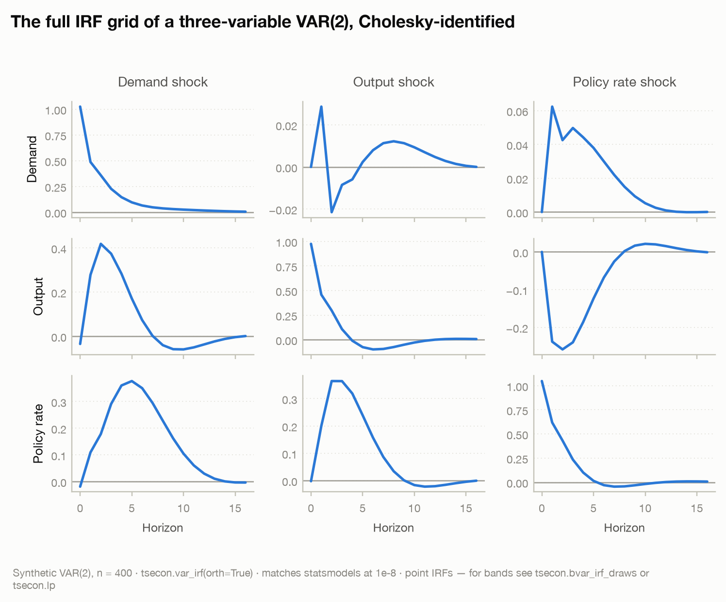
The figure — from the gallery's version of this same demand/output/policy-rate system — shows the full \(K \times K\) grid: rows are responding variables, columns are shocks. The estimated grid recovers the built-in story, including the near-zero response of demand to output shocks that the recursive ordering implies. Every array matches statsmodels at 1e-8.
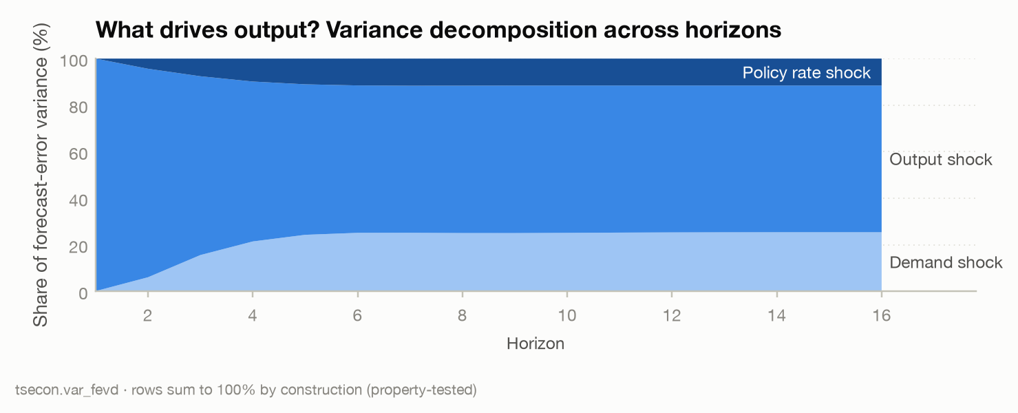
The companion summary is the forecast-error variance decomposition (FEVD): instead of tracing one shock's effect over time, it asks what share of each variable's forecast uncertainty each shock accounts for. With orthogonalized responses \(\Theta_h\), the share of shock \(j\) in variable \(i\)'s \(H\)-step forecast-error variance is
so each variable's shares sum to one at every horizon. Reading FEVDs is how you answer "is output mostly driven by its own shocks or by demand?" — and, at long horizons, "which shocks matter for the business cycle?"
fevd = tsecon.var_fevd(data, lags=1, horizon=16)
# Horizon-first, like var_irf: fevd[h][i][j] = share of variable i's
# (h+1)-step forecast-error variance attributed to shock j.  Rows sum to 1.
# (statsmodels' .fevd().decomp holds the same numbers variable-major —
# transpose (1, 0, 2) to compare.)
fevd[0][1]      # output at h=1:  [0.01, 0.99, 0.00] — own shock dominates on impact
fevd[15][1]     # output at h=16: [0.26, 0.73, 0.02] — demand grows to a quarter share
⚠ Common mistake. Reporting one Cholesky ordering and moving on. With \(K\) variables there are \(K!\) orderings; if your headline IRF survives only one of them, that is a finding about your assumption, not about the economy. At minimum, re-run
var_irfon reordered columns ofdataand confirm the responses you interpret are not artifacts of position. (The module roadmap ships an "all orderings" sensitivity helper precisely because almost nobody does this by hand — and order-invariant generalized IRFs, Pesaran and Shin 1998, as the alternative.)
Putting bands on the IRF
Every response above is a point estimate — one line per panel. But \(\hat\Phi_h\) is a nonlinear function of estimated coefficients, so each point carries sampling uncertainty, and a responsible IRF plot shades it. var_irf_bands is the banded companion to var_irf: it returns the identical [h][i][j] point path plus se, lower, and upper, by either of two routes. The asymptotic method (the default) uses the Lütkepohl (1990) delta method — the analytic derivative of the responses propagated through the coefficient covariance — and reports symmetric Wald bands \(\hat\Phi_{h,ij} \pm z_{1-\alpha/2}\,\widehat{\mathrm{se}}\). The bootstrap method resamples the fitted residuals, rebuilds and refits the VAR n_boot times, and reads percentile bands off the draws; bias_correct=True adds the Kilian (1998) bias correction that is the frequentist default for persistent data.
band = tsecon.var_irf_bands(data, lags=1, horizon=16, orth=True,
                            method="asymptotic", alpha=0.1)     # 90% bands
pt = np.asarray(band["point"]); lo = np.asarray(band["lower"]); hi = np.asarray(band["upper"])
for h in (0, 1, 4):                        # output (col 1) response to a demand shock (col 0)
    print(f"h={h:2d}  {pt[h,1,0]:+.3f}  90% band [{lo[h,1,0]:+.3f}, {hi[h,1,0]:+.3f}]")

boot = tsecon.var_irf_bands(data, lags=1, horizon=16, orth=True,
                            method="bootstrap", alpha=0.1, n_boot=2000, seed=0)
blo, bhi = np.asarray(boot["lower"]), np.asarray(boot["upper"])
print(f"bootstrap h=1 band [{blo[1,1,0]:+.3f}, {bhi[1,1,0]:+.3f}]")
h= 0  +0.079  90% band [+0.015, +0.144]
h= 1  +0.347  90% band [+0.280, +0.414]
h= 4  +0.092  90% band [+0.038, +0.146]
bootstrap h=1 band [+0.278, +0.415]
The delta-method SEs reproduce statsmodels' irf.stderr to machine precision; the bootstrap band lands on top of the asymptotic one here because the system is well-identified and nowhere near a unit root. Both routes carry the two flags through from var_irf: orth toggles Cholesky versus reduced-form responses — and the orthogonalized bands correctly pick up the extra term from differentiating the Cholesky factor \(P\) through \(\Sigma_u\), so they are not the reduced-form bands rescaled — while cumulative=True bands the running sum instead of the per-horizon response.
⚠ Common mistake. Reading a pointwise band as a joint one.
var_irf_bandscovers each horizon separately at level \(\alpha\); the probability that the entire response path stays inside the shaded region is smaller, and shrinks as you add horizons. The fix is a simultaneous (sup-\(t\)) band — Jordà (2009), Montiel Olea and Plagborg-Møller (2019) — and it now ships: passband="sup-t"to getsim_lower/sim_upper. On the audit's design a nominal 90% pointwise band holds the whole 13-horizon path 71.7% of the time and the sup-t band 85.2%. Unless you asked for the simultaneous band, describe the shaded region as "pointwise 90%", never "the path lies here with 90% probability".
Forecasting with a VAR
A fitted VAR forecasts by iteration: the one-step forecast plugs the last \(p\) observations into the estimated equations; the two-step forecast plugs in the one-step forecast where data are missing; and so on. Formally, with \(\hat y_{T+h|T}\) denoting the \(h\)-step forecast made at time \(T\),
The payoff over univariate forecasting is that each variable borrows strength from the others' histories — the rate's past helps predict output's future. Forecast-error variance accumulates through the same MA coefficients as the IRFs: the \(h\)-step forecast MSE matrix is \(\sum_{s=0}^{h-1} \Phi_s \Sigma_u \Phi_s'\), which grows with horizon and levels off (for a stable VAR) at the unconditional variance — long-horizon forecasts converge to the mean, and the intervals tell you how quickly your information decays.
fc = tsecon.var_forecast(data, lags=1, steps=8, alpha=0.05)
np.array(fc["point"])    # (steps x K): each row is one horizon, each column a variable
np.array(fc["lower"])    # 95% interval bounds, same shape
np.array(fc["upper"])
⚠ Common mistake. Treating these intervals as the whole truth. They account for innovation uncertainty (future shocks) under Gaussian errors, but not for parameter uncertainty — the fact that \(\hat A_1\) is itself an estimate. At short horizons in decent samples the difference is minor; at long horizons in small samples it is not, and the intervals are too narrow. The roadmap adds the Lütkepohl (2005, section 3.5) parameter-uncertainty correction and bootstrap intervals. And never report a VAR forecast without a benchmark: run
tsecon.accuracyagainst a naive forecast and test the difference withtsecon.dm_test(the forecast-evaluation chapter covers both).
Conditional forecasts: "if the policy rate stays on hold, what happens to output?"
The unconditional forecast answers "what does the model expect?". Policy institutions mostly ask a different question: what does the model expect for output if inflation follows this path and the policy rate stays on hold for two quarters? That is a conditional forecast — some cells of the future path are pinned, the rest are forecast given them — and it has a closed form (Doan, Litterman, and Sims 1984; Waggoner and Zha 1999). Stack the future innovations \(u = (u_{T+1}', \dots, u_{T+H}')'\); every future cell is the unconditional forecast plus a known linear combination of \(u\) (the MA coefficients \(\Phi_h\) again), so pinning \(m\) cells is a set of \(m\) linear constraints \(Bu = r\) on \(u\). Under Gaussian innovations the conditional path is the unconditional path plus the response to \(u^* = \Sigma B'(B \Sigma B')^{-1} r\) — the minimum-norm sequence of future shocks that delivers the conditions, which is also \(E[u \mid Bu = r]\) — and the conditional covariance is the unconditional one minus what the conditions explain. It is exactly what a Kalman smoother returns when the free future cells are set missing (Bańbura, Giannone, and Lenza 2015), which is how tsecon validates it: against statsmodels' VARMAX smoother, at 1e-8, on every fixture case.
H = 8
cond = np.full((H, data.shape[1]), np.nan)   # NaN = free; a number pins the cell
cond[:4, 2] = data[-1, 2]                    # the policy rate on hold for four quarters
cond[0, 0] = 0.5                             # plus a known demand-growth nowcast for h = 1
cf = tsecon.var_conditional_forecast(data, cond, lags=1, steps=H)
np.array(cf["point"])           # the conditional path; pinned cells hold their values exactly
np.array(cf["se"])              # 0 at pinned cells, smaller than cf["unconditional_se"] elsewhere
np.array(cf["shocks"])          # the implied future innovations the scenario needs
cf["mahalanobis_pvalue"]        # how hard the model is pushed: chi2(n_constrained) tail
The scenario pins five cells of this chapter's own system (columns: demand growth, output growth, policy rate). Output growth is never pinned, yet its standard error falls at every horizon — most at \(h = 2\) and \(h = 3\), to about 90% of the unconditional one — because output loads on both pinned series in \(A_1\) (0.3 on demand, \(-0.1\) on the rate), so the pinned paths carry information about it through the dynamics — and because later pins inform earlier innovations too. Conditioning tightens every free cell that shares innovations or dynamics with a pinned one, including horizons before the pinned one: the smoother runs backwards.
Read mahalanobis_pvalue before you read the path. It is the tail probability of the squared norm of the implied shocks under the model's own forecast distribution: a scenario the model would produce on its own scores near one, a scenario that needs a string of large same-signed innovations scores near zero — and the conditional forecast then describes a world the model finds implausible, not a likely one. Two further honest caveats: the intervals are innovation-uncertainty-only like var_forecast's (coefficients treated as known), and orth_shocks — the Waggoner-Zha structural version of the implied shocks — depends on the column ordering through the Cholesky factor, whereas the path and its covariance do not.
A policy desk rarely knows the rate path exactly, though. The policy rate expected at its current level with a 25bp standard deviation is a soft condition: condition_sd gives each conditioned cell a standard deviation (0 or NaN keeps it hard), and soft says what that standard deviation means. There is no default, because the two readings answer different questions:
sd = np.zeros((H, data.shape[1]))            # 0 = hard; a standard deviation > 0 makes the cell soft
sd[:4, 2] = 0.25                             # the rate at its current level, with a 25bp standard deviation
dens = tsecon.var_conditional_forecast(data, cond, lags=1, steps=H, condition_sd=sd, soft="density")
sig = tsecon.var_conditional_forecast(data, cond, lags=1, steps=H, condition_sd=sd, soft="signal")
With soft="density" (Andersson, Palmqvist, and Waggoner 2010) the scenario is a distribution: the rate's forecast at \(h = 1..4\) is \(N(\text{current level}, 0.25^2)\), so its point is the current level and its standard error exactly 0.25, the path is the hard conditional path, and every other cell's band widens by the uncertainty the scenario states — output growth's standard error at \(h = 3\) goes from 0.885 under the hard pin to 0.894. With soft="signal" (Monti 2010) the 25bp is the noise in a reading of the rate: the model weighs the readings against its own forecast, so the rate's conditional path moves off them (by up to 0.06, at \(h = 4\)) and its standard error, 0.215–0.230, is below the readings' 0.25. Use the density reading for a scenario you impose and the signal reading for information you observe with error; the mode key echoes which one you asked for. Interval conditions ("between 3% and 3.5%") and parameter uncertainty are not provided.
Residual diagnostics and lag order in one call each
Before any of this, the residuals have to be white. tsecon.var_diagnostics(data, lags=2, nlags=10) returns the multivariate Portmanteau statistic in both forms — portmanteau (Hosking's \(Q_h\)) and the small-sample portmanteau_adjusted (Lütkepohl 2005, section 4.4.3), each \(\chi^2(k^2(h - p))\) so nlags must exceed lags — three residual-normality tests — the multivariate Jarque-Bera with its skewness and kurtosis components (the residuals orthogonalized by the Cholesky factor of their covariance, the statsmodels convention, so the statistic depends on the column order as orthogonalized IRFs do), the same statistic on the symmetric root of the covariance (jarque_bera_symmetric, which is what JMulTi prints under the label "Doornik & Hansen (1994)": no transforms, and it changes when you change the units of a series), and the Doornik-Hansen (2008) omnibus test (doornik_hansen), which transforms each component's skewness and kurtosis to be close to normal in small samples and depends on neither the order nor the units — and the stability roots with the is_stable verdict. Report doornik_hansen: on Gaussian VAR(1) residuals with \(T = 40\) it rejected 5.3% of the time at a nominal 5% in tsecon's seeded Monte Carlo (2000 replications), where the asymptotic Jarque-Bera forms sit at 4.25–4.65%; its keys are None below eight observations, where the transform is undefined. For residuals from any other multivariate model — a VECM, a structural VAR — or for a single series, tsecon.multivariate_normality(resid) computes the same three tests. Report the adjusted Portmanteau at macro sample sizes: in tsecon's own seeded Monte Carlo (Gaussian VAR(1), \(k = 2\), \(T = 200\), nlags=8, 1000 replications) the unadjusted statistic rejects a true null 4.6% of the time and the adjusted one 5.4% at a nominal 5% — both within Monte-Carlo error here, with the unadjusted undersize growing as nlags becomes a larger fraction of \(T\). And choose the lag order on a common sample with tsecon.var_select_order(data, max_lags=8), which fits every candidate after dropping the same max_lags presample rows so the AIC/BIC/HQIC/FPE columns are comparable — reading aic off var_fit at different lags compares fits on different samples and can flip the ranking.
The drunk and her dog: cointegration
A drunk wanders home from the pub — a random walk, each step unrelated to the last, no tendency to return anywhere. Her dog wanders too: squirrels, lampposts, its own random walk. Track either path alone and it drifts unboundedly. But the dog is hers; when the gap gets too wide, she calls, and the dog trots back. Both paths are nonstationary, yet the distance between them is stationary — it gets stretched, then corrected, stretched, then corrected. That is cointegration (the fable is Murray 1994), and it describes an enormous amount of economics: consumption and income, short and long interest rates, spot and futures prices, prices of the same good in two cities. Theory says an equilibrium relationship tethers the pair; shocks displace it; economic forces pull it back.
First, the danger that makes this section necessary. Regress one independent random walk on another and OLS will routinely report a large t-statistic and a healthy \(R^2\) — the spurious regression problem (Granger and Newbold 1974; Yule was already worried in 1926). Both series trend somewhere; over any finite sample OLS obligingly finds a line relating the trends. The stationarity chapter's rule — difference unit-root series before regressing — exists to prevent exactly this. Watch it happen:
rng = np.random.default_rng(7)
T = 300
w1 = np.cumsum(rng.normal(size=T))       # a random walk
w2 = np.cumsum(rng.normal(size=T))       # an INDEPENDENT random walk
X = np.column_stack([np.ones(T), w2])
spur = tsecon.ols(w1, X, se_type="nonrobust")
spur["tvalues"][1]                       # t = 38.1 on a truly zero relationship
But differencing everything is a blunt instrument. If the series are cointegrated, the levels relationship is the economics, and differencing throws it away. Formally: \(y_t\) and \(x_t\), each I(1) (unit-root nonstationary), are cointegrated if some linear combination \(y_t - \beta x_t\) is I(0) (stationary). The vector \((1, -\beta)\) is the cointegrating vector — the leash. Equivalently, the two series share a single common stochastic trend (the drunk's path), and the combination that cancels it is stationary.
The Engle-Granger two-step test (Engle and Granger 1987) is the pedagogical and practical entry point. Step one: regress \(y\) on \(x\) in levels. Step two: test the residuals for a unit root. If the true relationship exists, OLS estimates \(\beta\) superconsistently — converging at rate \(T\) instead of the usual \(\sqrt{T}\) (Stock 1987), because any wrong \(\beta\) leaves a trending residual that OLS punishes enormously. If there is no cointegration, the residuals inherit the random walks and the unit root survives.
# A cointegrated pair sharing one stochastic trend:
trend = np.cumsum(rng.normal(size=T))            # the drunk
x = trend + rng.normal(size=T)                   # I(1)
y = 2.0 + 1.5 * trend + rng.normal(size=T)       # I(1), tethered to x

tsecon.check_stationarity(x)["quadrant"]         # "UnitRoot"
tsecon.check_stationarity(y)["quadrant"]         # "UnitRoot"

# Step 1: the cointegrating regression (levels on levels — legal HERE)
Xc = np.column_stack([np.ones(T), x])
step1 = tsecon.ols(y, Xc, se_type="nonrobust")
np.array(step1["params"])                        # [1.99, 1.48] — near the true (2, 1.5)
resid = y - Xc @ np.array(step1["params"])

# Step 2: unit-root test on the equilibrium error
eg = tsecon.adf(resid, regression="n")
eg["statistic"]                                  # -15.8: the residual is emphatically
                                                 # stationary -> cointegrated
⚠ Common mistake. Using standard ADF p-values in step two. The residuals are not raw data — OLS chose \(\hat\beta\) to make them as stationary-looking as possible, so the test statistic is biased toward rejection and needs stricter (more negative) critical values that depend on how many regressors were fitted (MacKinnon 2010 response surfaces; roughly \(-3.34\) at 5% for one regressor plus constant, versus \(-1.94\) for the raw no-constant ADF). Run step two on the spurious pair above and the standard machinery reports statistic \(-3.13\) with \(p = 0.002\) — a false detection of cointegration that the correct Engle-Granger critical value (\(-3.34\)) refuses. The \(-15.8\) in the genuine example clears any threshold; borderline values are exactly where the correction decides. You do not have to assemble the correction by hand:
tsecon.engle_granger(data, trend="c")runs both steps and returnsstat, a MacKinnonpvalue, and thecritsurface for the right number of regressors (statsmodels-exact at 1e-10 on the statistic), andtsecon.phillips_ouliarisgives the semiparametric \(Z_t\)/\(Z_a\) alternative, which trades the residual-ADF lag choice for a Bartlett long-run-variancebandwidth(Newey-West rule by default).
Super-consistency is about the point estimate; the standard errors of that step-one regression are another matter. Its limit distribution is not centred and not normal — serial correlation in the equilibrium error, and correlation between that error and the regressor's innovations, leave a second-order bias and a nuisance-parameter limit — so the OLS t-statistics are simply wrong, and no HAC correction fixes them. Three classical estimators remove the nuisance terms and give a mixed-normal estimator whose t-statistics are standard normal under the null: tsecon.fmols(y, x, trend="c") (Phillips-Hansen 1990 fully modified OLS, which corrects the regressand for endogeneity and subtracts the serial-correlation bias using the kernel long-run covariance of the residual system), tsecon.dols(y, x) (Stock-Watson 1993 dynamic OLS, which augments the regression with leads and lags of \(\Delta x_t\) chosen by BIC), and tsecon.ccr(y, x) (Park 1992 canonical cointegrating regression, which transforms the data instead). On the drunk-and-dog pair above all three agree with OLS to two decimals because the innovations are independent; on Wooldridge's T-bill-on-inflation data they move the slope from OLS's 0.64 to 0.74–0.85 and hand you a standard error of about 0.16 that means something. Each returns ols_params / ols_se beside its own params / se so the correction is visible, and each is arch-exact at 1e-10 (the model card lists the seeded Monte Carlo for size and super-consistency). They condition on cointegration — run engle_granger first.
Engle-Granger and the three corrected estimators all presume you already know the regressors are I(1). When you do not — a real interest rate that may or may not be stationary, a mix of trending and mean-reverting drivers — the ARDL bounds test of Pesaran, Shin and Smith (2001) asks the level question directly. Fit the autoregressive distributed lag model in error-correction form, \(\Delta y_t = \pi y_{t-1} + \sum_j \theta_j x_{j,t-1} + \text{lagged } \Delta\text{-terms} + \varepsilon_t\), and test \(\pi = \theta_1 = \dots = \theta_k = 0\) with an F statistic. Its null distribution depends on the integration order of the regressors, so PSS bound it: all-I(0) regressors give the lower critical values, all-I(1) the upper. Above the upper bound there is a level relationship whatever the regressors are; below the lower bound there is none; in between, it depends. tsecon.ardl_bounds_test(y, x) chooses the lag orders by BIC, runs the test (case 3, an unrestricted constant, by default) and returns the F, both bounds' critical values and p-values, a verdict, the long-run coefficients with standard errors, and the t statistic on \(y_{t-1}\) — which you must read too. On US consumption against income and the real rate (statsmodels' macrodata) the F is 4.89 with an upper-bound p-value of 0.046, a level relationship at 5%, while the t on lagged consumption is −1.61: the F is carried by the regressors' levels while consumption itself barely error-corrects, PSS's "degenerate case" that the F alone hides. One more warning, about the reference implementation: statsmodels 0.15's bounds_test reads the PSS table one row too far down (it counts \(y\) as a regressor) and reports \(p = 0.024\) on the same data; tsecon reads the right row, and the model card lays out the evidence — statsmodels' own simulator among it.
Cointegration is not just a diagnosis; it dictates the model. The Granger representation theorem (Engle and Granger 1987) says cointegrated systems admit — indeed require — an error-correction form:
Read it as the drunk-and-dog story in symbols: the term in parentheses is yesterday's disequilibrium — how far the dog had strayed — and \(\alpha < 0\) is the speed of adjustment, the fraction of the gap closed each period (\(\alpha = -0.3\): about 30% of any deviation corrected per quarter). Short-run dynamics live in the lagged differences; the long-run equilibrium lives in the levels term. No other specification in this book maps so directly onto economic language. The converse matters too: if the series are cointegrated, a VAR in differences omits the error-correction term and is misspecified — you would be modeling the dog while ignoring the leash.
For systems of \(K > 2\) variables, the questions multiply — there can be up to \(K - 1\) distinct cointegrating relationships, and Engle-Granger can only test one candidate at a time, dependent on which variable you normalize on. The system answer is the vector error-correction model (VECM) with Johansen's (1991) machinery. Rewrite the VAR in differences plus one levels term:
and everything hangs on the rank of \(\Pi\). Rank zero: no cointegration, difference and move on. Full rank \(K\): the levels were stationary all along. Rank \(r\) in between: exactly \(r\) cointegrating relationships, and \(\Pi\) factors as \(\alpha \beta'\), where the columns of \(\beta\) are the cointegrating vectors (the leashes) and \(\alpha\) holds each equation's adjustment speeds (who does the correcting). Johansen's trace and maximum-eigenvalue tests determine \(r\) sequentially, with the notorious practical wrinkle that five different conventions for deterministic terms (constants and trends inside or outside the equilibrium relation) give five different critical-value families — the classic cross-package replication trap.
Both the rank test and the VECM ship today (validated against statsmodels' coint_johansen and VECM). Here they are on a three-variable system built with two common stochastic trends, which leaves exactly one cointegrating relationship (rank \(r = K - \#\text{trends} = 3 - 2 = 1\)):
rng = np.random.default_rng(19)
T = 400
g1 = np.cumsum(rng.normal(size=T))                  # common stochastic trend 1
g2 = np.cumsum(rng.normal(size=T))                  # common stochastic trend 2
y1 = g1 + rng.normal(size=T)                        # I(1)
y2 = g2 + rng.normal(size=T)                        # I(1)
y3 = 0.5 * g1 - 0.8 * g2 + rng.normal(size=T)       # I(1), tethered to y1 and y2
coint_data = np.column_stack([y1, y2, y3])          # 400 x 3, one equilibrium relation

# Johansen: trace & max-eigenvalue rank tests (k_ar_diff = VAR lags minus one)
rank = tsecon.johansen(coint_data, k_ar_diff=2)
np.round(rank["trace_stat"], 1)                     # [134.0, 12.6, 0.6], tested sequentially
np.round(np.array(rank["trace_crit_90_95_99"])[:, 1], 1)   # 5% crit: [29.8, 15.5, 3.8]
rank["rank_trace_5pct"]                             # 1 — reject r=0, do NOT reject r<=1

# VECM at the selected rank: alpha (adjustment speeds), beta (cointegrating vectors).
# deterministic="co" (unrestricted constant) is the case johansen assumes; the
# default "n" (no deterministic terms) is a DIFFERENT model — on drifting data
# the two estimate visibly different betas, so match the case to the rank test.
vecm = tsecon.vecm(coint_data, k_ar_diff=2, coint_rank=1, deterministic="co")
np.round(np.array(vecm["beta"]).ravel(), 2)         # [1.0, -1.61, -2.01] — the leash, normalized
np.round(np.array(vecm["alpha"]).ravel(), 3)        # [-0.270, 0.142, 0.235] — who corrects
vecm["gamma"]                                       # short-run Gamma; also det_coef, sigma_u, llf
A few forces drive many series: dynamic factor models
Stack up the series a central bank watches — industrial production, payrolls, retail sales, PMIs, hundreds of them — and they visibly move together. Recessions are not a hundred independent events; they are one event observed a hundred noisy ways. The dynamic factor model (DFM) takes that observation literally: each observed series is a loading on a small number of common latent factors, plus an idiosyncratic remainder,
where \(f_t\) (dimension 2–10, say, against \(N\) in the hundreds) itself follows a VAR. The factors are "the state of the economy" as the panel sees it; the loadings \(\lambda_i\) say how each series reads it. Estimation is a beautiful piece of recycling: principal components consistently recover the factor space when \(N\) and \(T\) are both large (Stock and Watson 2002), and the state-space/Kalman machinery from the state-space chapter — the same engine as tsecon.local_level_smooth — refines the estimates, handles missing observations natively, and copes with the "ragged edge" of data releases that makes DFMs the backbone of institutional nowcasting (that chapter takes over from here).
Factors also rescue structural analysis. A three-variable VAR asks the impulse-response question inside a tiny information set; the FAVAR (factor-augmented VAR; Bernanke, Boivin, and Eliasz 2005) runs the VAR on (factors, policy rate) and then maps the responses back through the loadings — one monetary-policy shock, impulse responses for hundreds of series, and a partial answer to the omitted-information critique of small VARs.
Both objects in this section ship. tsecon.factor_model extracts the principal-component factors and answers the how many question (Bai-Ng and Ahn-Horenstein), and tsecon.favar fits the two-step Bernanke-Boivin-Eliasz FAVAR including the slow/fast rotation — the two sections at the end of this chapter work through both. The ragged-edge nowcasting member, tsecon.dfm_nowcast (Doz-Giannone-Reichlin two-step, plus a method="mle" route) with its tsecon.dfm_news revision decomposition, belongs to Chapter 11, which takes over from here. What is still module-spec material is the wider DFM facade: mixed frequencies, arbitrary interior missing-data patterns, and EM estimation.
When the system gets big
Count parameters: a VAR(p) on \(K\) variables estimates \(K(1 + pK)\) coefficients.
| System | \(K\) | \(p\) | Coefficients | Typical \(T\) |
|---|---|---|---|---|
| Small quarterly VAR | 3 | 4 | 39 | 250 |
| Medium macro VAR | 8 | 4 | 264 | 250 |
| Monthly financial system | 20 | 13 | 5,220 | 700 |
| "Model the whole panel" | 100 | 4 | 40,100 | 700 |
Past the second row, OLS is drowning — thousands of coefficients from hundreds of observations means wildly noisy estimates, and beyond it the regression is not even computable. This is the curse of dimensionality, and modern practice offers three escapes. Compress: the factor models above replace \(K\) series with a handful of factors. Shrink: Bayesian VARs pull coefficients toward a disciplined prior — each series a near-random-walk, distant lags near zero (the Minnesota prior; Litterman 1986) — and with the shrinkage tuned properly a 100-variable BVAR forecasts remarkably well (Bańbura, Giannone, and Reichlin 2010); that is Chapter 10. Regularize: lasso-type penalties zero out most coefficients, with lag-aware penalty structures shrinking distant lags harder; that is Chapter 12. The three are complements, not rivals — big institutional models routinely shrink and compress.
The frontier
Where research-grade practice currently stands, and where the module roadmap points:
- IRF inference is the active battleground. The naive asymptotic bands of the 1980s undercover badly for persistent data. Kilian (1998) made bias-corrected bootstrap-after-bootstrap bands the frequentist standard; Gonçalves and Kilian (2004) extended validity to conditional heteroskedasticity via the wild bootstrap; and Brüggemann, Jentsch, and Trenkler (2016) proved a sharp negative result — for statistics that depend on \(\Sigma_u\) (that is, all Cholesky IRFs and FEVDs), even the wild bootstrap is invalid under conditional heteroskedasticity, and only a moving-block bootstrap of residual vectors survives. Almost no mainstream library implements this correctly; the roadmap makes it a default, feasible because the Rust core makes double bootstraps cheap.
- Pointwise bands are the wrong object anyway. Readers interpret an IRF band as covering the whole path, but pointwise bands cover one horizon at a time. Montiel Olea and Plagborg-Møller (2019) supply sup-t simultaneous bands, and this is now literally a one-flag fix:
band="sup-t". It corrects the multiplicity exactly; it does not repair a standard error that was already short, which is why the measured sup-t rate lands at 85.2% rather than 90%. - Persistence poisons long horizons. With the largest root near one, standard bands (bootstrap included) undercover at long horizons; Inoue and Kilian (2020) develop uniformly valid procedures. The roadmap's stance: at minimum, warn loudly when the largest companion root exceeds ~0.97 and horizons are long.
- VARs versus local projections — the loudest methods debate of the last decade — was largely settled by Plagborg-Møller and Wolf (2021): in population they estimate the same impulse responses; in samples the trade is bias (LP) versus variance (VAR). The local-projections chapter takes this up.
- Cointegration testing under real-world errors. Asymptotic Johansen tests over-reject under heteroskedasticity; Cavaliere, Rahbek, and Taylor (2012) supply wild-bootstrap rank tests — bootstrapped under the restricted rank, which is the part home-rolled code gets wrong. Meanwhile much of the ecosystem still uses table-lookup p-values instead of MacKinnon-Haug-Michelis (1999) response surfaces.
- Spillovers and networks. Diebold and Yilmaz (2012, 2014) turned the generalized FEVD into connectedness measures now ubiquitous in empirical finance — with a hidden trap that
tsecon.connectednessmakes explicit rather than hiding: GFEVD rows do not sum to one, and competing normalizations silently change the numbers, so the function states which one it applies (the standard 2012 row-normalization). The last section of this chapter works it through. - Honest open problems: inference on impulse responses that is simultaneously robust to persistence, heteroskedasticity, and long horizons; propagating cointegration-rank uncertainty into downstream VECM inference instead of conditioning on the tested rank; and valid post-selection inference (e.g., Granger causality after lasso) in high-dimensional systems (Hecq, Margaritella, and Smeekes 2023).
Which method when
| Situation | Reach for | Because |
|---|---|---|
| Joint dynamics of 2–8 stationary series | var_fit + var_irf/var_fevd |
The workhorse: symmetric treatment, readable dynamics, no incredible restrictions |
| "Does \(x\) help predict \(y\)?" | var_granger |
The precise version of the question — predictive content, tested; write "predicts," not "causes" |
| Short-horizon forecasts of several related series | var_forecast |
Each variable borrows strength from the others' histories; benchmark it with accuracy/dm_test |
| "If inflation follows this path, what happens to output?" | var_conditional_forecast |
The Doan-Litterman-Sims / Waggoner-Zha closed form; read mahalanobis_pvalue first to see how hard the model is pushed. A path known only up to a standard deviation: condition_sd= with soft="density" (a scenario you impose) or soft="signal" (a noisy reading) |
| Are the residuals white and Gaussian, is the system stable, which lag order? | var_diagnostics, var_select_order (multivariate_normality for any residual matrix) |
Adjusted Portmanteau, Doornik-Hansen normality (order- and unit-free; the Cholesky and JMulTi Jarque-Bera forms alongside), stability roots; common-sample AIC/BIC/HQIC/FPE |
| Unit-root series with no equilibrium tie | Difference, then VAR | Levels regressions between untethered I(1) series are spurious |
| I(1) series theory says move together | engle_granger (or phillips_ouliaris) |
Superconsistent \(\beta\), direct test of the equilibrium, MacKinnon p-values already applied; simplest credible check for one relationship |
| One equilibrium relation, and you need standard errors on its coefficients | fmols (or dols / ccr) |
The static OLS is superconsistent but its t-statistics are invalid; the fully modified / dynamic / canonical corrections make them standard normal — after engle_granger has confirmed cointegration |
| One candidate equilibrium, but the regressors' integration order is unclear or mixed | ardl_bounds_test |
The PSS bounds test holds whether each regressor is I(0) or I(1); read the F's upper-bound p-value and the t on \(y_{t-1}\) |
| Several I(1) series, unknown number of equilibria | johansen, then vecm at the selected rank |
System estimation of the rank and all cointegrating vectors, plus adjustment speeds — match deterministic= to the case the rank test assumed |
| "What does a policy shock do?" | Cholesky var_irf today; Chapter 8 for real identification |
Ordering is an assumption — defend it or replace it with structural restrictions |
| Hundreds of series, one underlying cycle | factor_model (how many, and the factors), then favar if you need one identified shock |
A few factors capture the comovement; favar maps the shock back to every series in the panel |
| Same panel, but read in real time off a ragged edge | dfm_nowcast/dfm_news (Chapter 11) |
Kalman machinery handles missing data and ragged edges, and attributes each revision to the release that caused it |
| \(K\) too big for OLS but a VAR is the right object | Bayesian shrinkage (Chapter 10) or lasso-type penalties (Chapter 12) | Discipline from priors or penalties beats unrestricted noise |
What tsecon implements today
Available now in Python (validated against statsmodels at 1e-8):
tsecon.var_fit(data, lags=2, trend="c")— equation-by-equation OLS estimation; returnsparams(rows: constant, then stacked lag coefficients; columns: equations),sigma_u,llf,aic/bic/hqic, and a characteristic-root stability summarytsecon.var_irf(data, lags=2, horizon=10, orth=True, trend="c")— impulse responses,irf[h][i][j];orth=Falsegives the raw MA coefficients \(\Phi_h\)tsecon.var_fevd(data, lags=2, horizon=10, trend="c")— variance decompositions, horizon-first like the IRFs:fevd[h][i][j]tsecon.var_forecast(data, lags=2, steps=8, alpha=0.05, trend="c")— iterated point forecasts with innovation-uncertainty intervalstsecon.var_granger(data, caused, causing, lags=2, trend="c")— block F test, group-to-grouptsecon.var_conditional_forecast(data, conditions, lags=2, trend="c", steps=None, alpha=0.05, condition_sd=None, soft=None)— conditional forecasts (Doan-Litterman-Sims / Waggoner-Zha): the conditionalpointpath, per-horizoncov/se, the impliedshocks/orth_shocks, and amahalanobis_pvalueplausibility check;condition_sdwithsoft="density"(Andersson-Palmqvist-Waggoner) orsoft="signal"(Monti) makes conditions Gaussian-soft; validated against the closed form and statsmodels'VARMAXsmoother (with a measurement-noise covariance for the signal reading)tsecon.var_diagnostics(data, lags=2, trend="c", nlags=10)— Portmanteau (unadjusted and adjusted), multivariate Jarque-Bera with skewness/kurtosis components (Cholesky and symmetric-root forms; the latter reproduces JMulTi's "Doornik & Hansen (1994)" block), the Doornik-Hansen (2008) omnibus normality test, stability rootstsecon.multivariate_normality(resid)— the same three normality tests on any \(T \times k\) residual matrix, or on one series (the univariate Doornik-Hansen test)tsecon.var_select_order(data, max_lags=8, trend="c")— common-sample AIC/BIC/HQIC/FPE lag-order selectiontsecon.johansen(data, k_ar_diff=2)— Johansen trace and maximum-eigenvalue rank tests (unrestricted-constant convention, statsmodelsdet_order=0), returningtrace_stat/max_eig_stat, the_90_95_99critical-value tables, the impliedrank_trace_5pct/rank_max_eig_5pct, and the eigenvectorsevectsecon.vecm(data, k_ar_diff=2, coint_rank=1, deterministic="n", seasons=0)— ML VECM estimation:alpha,beta,det_coef_coint,gamma,det_coef,sigma_u,llf(statsmodels-exact).deterministictakes all nine statsmodels cases:"n"(no deterministic terms, the default),"co"(unrestricted constant — the casejohansenassumes; use it when the rank came fromjohansen), the restricted"ci"/"li"(constant/trend inside the cointegration relation — their coefficients widen the cointegrating matrix and come back asdet_coef_coint),"lo", and the combinations"colo"/"coli"/"cilo"/"cili";seasons=/first_season=add centered seasonal dummiestsecon.engle_granger(data, trend="c", autolag="aic")— the two-step residual cointegration test with MacKinnon p-values and critical values already applied (column 0 is the regressand; do not add your own constant), andtsecon.phillips_ouliaris(y, x, trend="c", test_type="Zt")for the semiparametric \(Z_t\)/\(Z_a\) alternativetsecon.fmols(y, x, trend="c", kernel="bartlett", bandwidth=None),tsecon.dols(y, x, lags=None, leads=None, ic="bic"),tsecon.ccr(y, x)— Phillips-Hansen fully modified OLS, Stock-Watson dynamic OLS and Park canonical cointegrating regression of one cointegrating vector with valid (mixed-normal) inference:params/se/tvalues/pvalueson the regressors and deterministics, the long-run covariance pieces (omega/lambda/sigma), thebandwidthused (automatic bybandwidth_rule="newey-west"or"andrews"), DOLS's selectedlags/leads, andols_params/ols_sefor comparison (arch-exact at 1e-10)tsecon.ardl_bounds_test(y, x, lags=None, order=None, case=3, ic=None)— the ARDL / unrestricted error-correction model and the Pesaran-Shin-Smith (2001) bounds test for a level relationship: the F (statistic) and the t on \(y_{t-1}\) (t_statistic), the I(0)/I(1) critical values (crit_lower/crit_upper) and p-values (p_value_lower/p_value_upper) at the number of regressors, averdict, the long-run coefficients (long_run, delta-methodlong_run_se) and BIC/AIC/HQIC lag-order selection (statsmodels-exact at 1e-10 on the estimates; the F at 1e-10 against an exact-rational referee, statsmodels' own two F routes carrying up to 1.4e-9 of rounding; statsmodels' table-key andnobsdefects are documented, not inherited)tsecon.var_irf_bands(data, ...)— the banded companion tovar_irf: Lütkepohl delta-method or residual/Kilian-bias-corrected bootstrap bands, andband="sup-t"/"sidak"/"bonferroni"for simultaneous bands over aband_scopeyou choose and it reports backtsecon.connectedness(data, lags=2, horizon=10, trend="c")— the Diebold-Yilmaz spillover table off the row-normalized generalized FEVD (last section of this chapter)tsecon.factor_model(panel, n_factors=2, kmax=8)— PCA factors,eigenvalues, the Bai-Ngicp1/icp2/pcp1/pcp2counts and the Ahn-Horensteiner/er_ratiostsecon.favar(panel, policy, n_factors=2, lags=2, horizon=16, slow_indices=None)— the two-step Bernanke-Boivin-Eliasz FAVAR, returningirf_panel(\(N \times (H+1)\)) andirf_policytsecon.historical_decomposition(...)andtsecon.structural_fevd(...)— per-(time, variable, shock) contributions and a FEVD for any structural impact matrix, not just Cholesky (Chapter 8 uses both)- Supporting cast used in this chapter:
check_stationarity,adf,kpss,ols,ljung_box,long_run_variance
Built in Rust, awaiting Python bindings (in the tsecon-var crate): the joint cross-horizon forecast-error covariance (forecast_error_cov_joint) as a matrix of its own — the sup-t forecast band uses it internally. The per-horizon forecast MSE matrices that used to sit here are bound as of 0.11 as var_forecast(...)["cov"], with Lütkepohl's parameter-uncertainty term under param_uncertainty=True (see the VAR card); the common-sample lag-order selection and the stability accessors as of 0.10.0 (var_select_order, var_diagnostics).
Roadmap (Module 04 — Multivariate Models): MacKinnon-Haug-Michelis p-values and Bartlett small-sample correction for the shipped Johansen tests, plus VECM restriction testing; Toda-Yamamoto causality; the remaining bootstrap IRF schemes (Gonçalves-Kilian wild and Brüggemann-Jentsch-Trenkler moving-block, beyond the shipped residual and Kilian-bias-corrected ones); generalized IRFs as a standalone call (the generalized FEVD already ships inside connectedness); the wider DFM facade — mixed frequencies, interior missing data, EM; VARX/VARMA; Markov-switching and smooth-transition VARs (threshold_var/threshold_var_test and the threshold VECM threshold_vecm/hansen_seo_test ship — Chapter 13 — and star is univariate, not a system STVAR); global VARs (the mean-group panel VAR ships as mean_group_var, Chapter 14).
Three worked out in full: connectedness, factors, and FAVAR
tsecon.connectedness, tsecon.factor_model, and tsecon.favar each ship with Python bindings and a golden fixture, and each rewards more than a one-line entry in the list above. The three sections that follow are the working chapter for them — the intuition, the estimator, the call, and the traps.
Connectedness: who spills over to whom (Diebold-Yilmaz)
You already have the FEVD. It answers, variable by variable, what share of this series' forecast uncertainty comes from that series' shocks? Francis Diebold and Kamil Yilmaz's move (2012, 2014) was to stop reading the FEVD one row at a time and read the whole matrix as a weighted directed network: variable \(j \to\) variable \(i\) with weight equal to the FEVD share. Collapse that network to a single number — the fraction of total forecast-error variance that crosses variable boundaries — and you have a connectedness index you can compute on a rolling window and watch spike when a crisis hits. That one plot, spillovers climbing into 2008 and again into 2020, is now a fixture of empirical finance and systemic-risk monitoring.
The estimator starts from a VAR(p) but deliberately does not use the Cholesky FEVD, because Diebold-Yilmaz want a table that does not flip when you reorder the variables. They use the generalized FEVD (Pesaran and Shin 1998; Koop, Pesaran, and Potter 1996), which measures the effect of a shock to variable \(j\) without orthogonalizing — each variable gets its "own" shock, correlated with the others, integrated over the system's response:
where \(e_i\) selects variable \(i\) and \(\Phi_h\) are the MA coefficients from the IRF section. Order-invariance is the payoff; the price is the trap the frontier section flagged — the rows of \(\theta\) do not sum to one, because generalized shocks are not orthogonal. So Diebold-Yilmaz normalize each row, \(\tilde\theta_{ij} = \theta_{ij} / \sum_{k} \theta_{ik}\), and read the resulting table:
- Total connectedness \(C = 100 \times \frac{1}{K}\sum_{i \neq j} \tilde\theta_{ij}\) — the average share of a variable's forecast-error variance that comes from other variables.
- Directional TO others (column off-diagonal sums): how much each variable transmits.
- Directional FROM others (row off-diagonal sums): how much each variable receives.
- Net = TO − FROM: positive marks a net transmitter, negative a net receiver.
- Pairwise net \(\tilde\theta_{ji} - \tilde\theta_{ij}\): the net flow along each edge.
Reach for connectedness when you have several — or many — series and want a scalar (or a rolling series) summarizing how linked the system is, plus a directional ranking of who drives whom. It is the readable summary the full \(K \times K\) IRF grid cannot be past a handful of variables, and unlike a Cholesky FEVD it does not depend on an ordering you would have to defend.
import json, numpy as np, tsecon

var = json.load(open("fixtures/var.json"))
data = np.array(var["data_100dlog_gdp_cons_inv"])   # 202 x 3: growth of GDP, consumption, investment

c = tsecon.connectedness(data, lags=2, horizon=10, trend="c")
round(c["total"], 1)             # 44.8 — ~45% of the system's forecast-error variance is cross-series
np.round(c["net"], 1)            # [ 1.4, 6.8, -8.2 ]: consumption a net transmitter, investment a net receiver
np.round(np.array(c["gfevd"]), 2)
# [[0.46, 0.30, 0.24],          <- GDP: 46% own shocks, the rest from cons & inv
#  [0.27, 0.71, 0.03],          <- consumption is mostly self-driven (smooth series)
#  [0.32, 0.20, 0.49]]          <- investment absorbs a lot from GDP and consumption
np.round(np.array(c["pairwise_net"]), 1)[1, 2]   # 5.7 — the dominant edge: consumption -> investment
Read the table like a balance sheet. The normalized gfevd rows each sum to one; the diagonal is the own-shock share and the off-diagonal is what leaks in. Consumption's row is 71% own — smooth series forecast themselves — while investment's row shows only 49% own, the rest imported. That asymmetry is exactly what net reports: consumption's +6.8 makes it the system's largest net transmitter of forecast-error variance and investment's -8.2 the largest net receiver, with the single strongest edge (pairwise_net[1,2] = 5.7) running consumption \(\to\) investment. The headline total = 44.8 says nearly half of the three-variable system's forecast uncertainty is cross-series rather than own — a moderately connected system. These numbers reproduce the fixtures/connect.json golden to the digit.
⚠ Common mistake. Reporting one full-sample connectedness number as if it were the finding. Diebold-Yilmaz connectedness earns its keep rolling — estimated on a moving window so you can see total and net connectedness climb in stress episodes; a single static number averages that dynamics away. Two more traps: the row-normalization is a choice (competing normalizations of the generalized FEVD change the numbers, so state which you used —
tseconuses the standard Diebold-Yilmaz 2012 row-normalization), and connectedness is a reduced-form object. It inherits the VAR's specification (lags, horizon, variable set) and the generalized FEVD's non-orthogonality; it describes forecast-error-variance linkage, not causation. And valid error bands are genuinely hard here — because every entry depends on \(\Sigma_u\), the Brüggemann-Jentsch-Trenkler (2016) warning from the frontier applies in full.
How many factors? Bai-Ng and Ahn-Horenstein
The dynamic-factor section promised that a handful of common forces drive a big panel. Before you can estimate them you have to answer the question a scree plot only gestures at: how many factors? Pick too few and the omitted comovement leaks into the idiosyncratic errors; pick too many and you are modeling noise. factor_model extracts the factors by principal components and returns two families of formal answers to the count.
Principal components on a standardized \(T \times N\) panel recover the factor space consistently as \(N\) and \(T\) both grow (Stock and Watson 2002): the leading eigenvectors are the loadings, the scaled leading components are the factors. The count comes from two ideas. Bai and Ng (2002) treat it as model selection — the residual variance \(V(k)\) falls as you add factors, so trade it against a penalty \(g(k)\) that must vanish slower than \(1/\min(N,T)\):
and choose the minimizing \(k\) (the function returns icp1/icp2/pcp1/pcp2, the four penalty variants). Ahn and Horenstein (2013) exploit a sharper fact: a genuine factor's eigenvalue grows like \(N\), an idiosyncratic one stays \(O(1)\), so the ratio of adjacent ordered eigenvalues \(ER(k) = \mu_k/\mu_{k+1}\) spikes at the true number. Take the argmax (er). The eigenvalue ratio needs no penalty tuning, which is why it holds up when \(N\) is only moderate — exactly the regime where the Bai-Ng penalties, built for large \(N\), wobble.
fav = json.load(open("fixtures/favar.json"))
panel = np.array(fav["X_standardized"]).T           # 300 x 24, standardized (T x N); true r = 2

fm = tsecon.factor_model(panel, n_factors=2, kmax=8)
np.round(np.array(fm["eigenvalues"])[:5], 2)   # [11.09, 9.01, 0.79, 0.56, 0.36] — a clean two-factor cliff
fm["er"]                                         # 2  — Ahn-Horenstein eigenvalue ratio nails the true rank
np.round(np.array(fm["er_ratios"])[:3], 1)       # [1.2, 11.4, 1.4] — the ratio spikes at k = 2
fm["icp2"], fm["pcp2"]                            # (7, 8) — Bai-Ng OVERSELECTS here: N = 24 is small
The scree tells the story at a glance: two eigenvalues of order 10, then a fall off a cliff to 0.79 — a textbook two-factor panel, which is what the fixture's DGP built. The Ahn-Horenstein ratio makes the cliff a number: er_ratios peaks at \(k=2\) with value 11.4 (that is \(9.01/0.79\)), and er returns 2. The Bai-Ng criteria, by contrast, report 7 and 8 — they overselect badly, and if you sweep kmax you will watch icp2 track it upward. That is not a bug; it is Bai-Ng's large-\(N\) asymptotics failing at \(N=24\), precisely the small-panel pathology Ahn and Horenstein designed the ratio to survive. When the two families disagree, trust the eigenvalue cliff and the ratio in small \(N\), the penalized criteria when both dimensions are large.
⚠ Common mistake. Reading a single PCA factor as if it were a structural object — "factor 1 is the business cycle." Factors are identified only up to rotation (PCA pins them to orthonormal, up to a sign), so an individual factor and its loadings have no intrinsic meaning; only the space they span, and quantities invariant to rotation (fitted values, the panel IRFs of the next section), are estimable. Two neighboring traps: forgetting to standardize the panel, which lets a few high-variance series masquerade as factors, and treating Bai-Ng's number as gospel at modest \(N\) — as the code just showed, it can be off by a factor of three. Static PCA also ignores the factors' own serial correlation; the state-space refinement in Chapter 4 recovers it and handles missing data and ragged edges (Chapter 11).
FAVAR: one policy shock, hundreds of responses
Here is the complaint that motivates the whole method. A three-variable VAR asks "what does a monetary-policy shock do?" inside an information set of three series — while the central bank, and everyone trading against it, watches hundreds. That mismatch has a name and a symptom: the small VAR is plausibly non-fundamental (its shocks are not the economy's shocks), and it produces the notorious price puzzle, prices rising after a contractionary shock, an artifact of omitted information about future inflation. Bernanke, Boivin, and Eliasz (2005) close the gap without estimating a 200-variable VAR: summarize the big panel with a few factors, run the VAR on (factors, policy rate), identify the policy shock there, and then map the response back through the loadings to every series in the panel. One shock, hundreds of impulse responses.
It is a two-step estimator. Step one extracts \(r\) factors \(\hat F_t\) from the informational panel by principal components — the factor_model machinery above. Because those factors are contaminated by the contemporaneous policy rate, a recursive identification needs them cleaned: BBE regress the factors on the "slow-moving" variables (output, prices — things that do not respond to policy within the period) and the policy rate, and keep the part spanned by the slow variables (slow_indices). Step two fits a VAR(p) on \(Y_t = (\hat F_t', R_t)'\) with the policy rate ordered last, so a Cholesky shock to the final equation (orth=True) is the recursive monetary-policy shock — the rate reacts to the factors within the quarter, but the factors do not react to the rate until the next. The observation equation \(X_t = \Lambda \hat F_t + \dots\) then turns the factor IRF into a panel IRF, \(\text{IRF}^X_h = \Lambda\,\text{IRF}^F_h\): irf_panel is \(N \times (H+1)\), one row per observed series, and irf_policy is the rate's own response.
Reach for a FAVAR when the structural question genuinely needs a large information set — to kill the price puzzle, to read responses for many disaggregated series off one identified shock, or to condition on a rich dataset without the parameter count of a full BVAR. The alternatives sit on either side: a small SVAR (Chapter 8) when a handful of variables suffice, a Minnesota-shrinkage BVAR (Chapter 10) when you want to keep every series but discipline the coefficients, local projections (Chapter 9) when you want a single response with fewer functional-form commitments. FAVAR is the specific combination factor compression + recursive identification.
# A FAVAR DGP with a real transmission channel: a contractionary rate cools the
# common factors with a lag; the rate reacts to the factors (a Taylor-rule feedback);
# a 40-series panel loads on the factors.
rng = np.random.default_rng(11)
T, burn, N = 400, 100, 40
Phi = np.array([[0.6, 0.05], [0.0, 0.5]])           # factor own-dynamics
Psi = np.array([-0.5, -0.3])                        # lagged rate -> factors (cooling)
rho, theta = 0.7, np.array([0.15, 0.10])            # policy AR + reaction to lagged factors
F = np.zeros((T + burn, 2)); R = np.zeros(T + burn)
for t in range(1, T + burn):
    F[t] = Phi @ F[t - 1] + Psi * R[t - 1] + rng.normal(size=2) * [1.0, 0.8]
    R[t] = rho * R[t - 1] + theta @ F[t - 1] + rng.normal() * 0.5
F, R = F[burn:], R[burn:]
L = rng.normal(size=(N, 2))                          # panel loadings
X = F @ L.T + rng.normal(size=(T, N)) * 0.5          # T x N informational panel
Xs = (X - X.mean(0)) / X.std(0)                      # standardize (PCA convention)

res = tsecon.favar(Xs, R, n_factors=2, lags=2, trend="c", horizon=16, orth=True)
res["n_endog"], res["policy_index"]     # (3, 2): the VAR is [F1, F2, R] with the rate ordered last
np.round(np.array(res["irf_policy"])[[0, 1, 2, 4, 8]], 3)   # [0.517, 0.359, 0.207, -0.004, -0.048]
# Two panel series with opposite-signed loadings on factor 1:
irf_panel = np.array(res["irf_panel"])
np.round(irf_panel[int(np.argmax(L[:, 0]))][[0, 2, 4, 8]], 3)   # [0.0, -0.228, -0.187, -0.004]
np.round(irf_panel[int(np.argmin(L[:, 0]))][[0, 2, 4, 8]], 3)   # [0.0,  0.200,  0.175,  0.010]
Read the responses through the identification. irf_policy starts at 0.517 — the Cholesky impact of the shock on the rate's own equation, positive by construction — and decays with a mild overshoot, the rate's own dynamics. The panel IRFs all start at exactly zero on impact: the panel moves only through the factors, and under the recursive ordering the factors do not respond to the policy shock within the period. From \(h=1\) they build up, and the sign follows the loading — the series that loads most positively on factor 1 falls (\(-0.23\) at \(h=2\)) as the contractionary shock cools the common factor, while the series that loads most negatively rises (\(+0.20\)). That is the entire FAVAR payoff in one panel: a single identified shock, disaggregated onto every series with the right sign and shape. The factor-extraction step is not taken on faith — fixtures/favar.json pins it against numpy's PCA, and the FAVAR's step-one factors reproduce those principal components up to a sign flip.
⚠ Common mistake. Forgetting that the recursive ordering is the identifying assumption. Ordering the rate last says the factors (and the slow variables behind them) do not react to policy within the period, while policy reacts to everything — defensible for a monthly or quarterly policy rate, but an assumption to argue, not a computation, exactly as in Chapter 8; change the ordering or the slow/fast split and the shock changes. Two more: do not interpret an individual factor's IRF (the factors are identified only up to rotation — but the panel IRFs \(\Lambda \hat F\) are rotation-invariant, which is the whole reason BBE map back to observables), and do not trust asymptotic error bands. The factors are generated regressors, so honest inference must bootstrap the two-step procedure — factor extraction and VAR together — and account for the estimation of \(\hat F\) (Bai and Ng 2006); bands that condition on \(\hat F\) as if it were data are too narrow.
Further reading
- Sims (1980), "Macroeconomics and Reality," Econometrica — the manifesto: why "incredible" identifying restrictions should give way to VARs; still the best statement of the research program this chapter serves.
- Granger (1969), Econometrica — defines Granger causality as testable predictive content; read alongside its misuses.
- Granger & Newbold (1974), Journal of Econometrics — the spurious-regression bombshell: high \(R^2\) and t-statistics from independent random walks.
- Engle & Granger (1987), Econometrica — cointegration, the two-step test, and the Granger representation theorem in one Nobel-cited paper.
- Johansen (1991), Econometrica — system maximum-likelihood cointegration: rank tests and the VECM; the machinery behind every "johansen" function ever shipped.
- Murray (1994), The American Statistician, "A Drunk and Her Dog" — two pages that teach cointegration and error correction better than most textbook chapters.
- Stock & Watson (2002), Journal of the American Statistical Association — principal-components factor estimation for large panels; the foundation of modern DFM and nowcasting practice.
- Bernanke, Boivin & Eliasz (2005), Quarterly Journal of Economics — the FAVAR: factor-augmented VARs as the answer to small-VAR information sets.
- Lütkepohl (2005), New Introduction to Multiple Time Series Analysis — the reference on everything reduced-form in this chapter; the library validates against its worked examples.
- Kilian & Lütkepohl (2017), Structural Vector Autoregressive Analysis — the modern graduate treatment of identification and inference; the bridge from this chapter to Chapter 8 and the frontier.