Chapter 3 — Honest Inference with Dependent Data¶

Part of The tsecon Guide to Time Series Econometrics. Chapters mirror the library's modules; code runs against the current Python API unless marked otherwise.

Prerequisites: Chapters 1–2 (autocorrelation, the ACF, stationarity), plus OLS regression and the idea of a standard error.

You will learn:

Why autocorrelation makes textbook standard errors too small — and how to think about it as a loss of effective sample size
The long-run variance: the one number that repairs the variance of any time series average
The robust standard-error ladder — iid → HC0/HC1 → HAC — and how to climb it with tsecon.ols(se_type=...)
Modern fixed-b and EWC inference (Lazarus–Lewis–Stock–Watson 2018), and why it exists
Block and wild bootstraps that respect dependence, with Monte Carlo experiments that reproduce exactly on any machine
Quantile regression: inference on the conditional distribution rather than the mean — the check loss, when quantile slopes fan apart, and the Powell sandwich

The idea¶

Suppose you regress quarterly inflation on a measure of labor-market slack, fifty years of data, 200 observations. The coefficient comes out negative, the t-statistic is 3.5, and the textbook says anything above 2 is significant. Should you believe it?

Probably not — and the problem is not the coefficient. It is the denominator of that t-statistic. The textbook standard-error formula divides by the square root of the sample size, and in doing so it assumes that each of your 200 quarters is a fresh, independent piece of news. But inflation in the second quarter of 1985 looks a great deal like inflation in the first quarter of 1985. So does slack. Each new observation mostly repeats what the previous one already told you.

Here is an analogy. You want to know the average political opinion in a country, and you survey 200 people — but all of them live on the same street. You have 200 responses, yet nothing like 200 independent opinions: neighbors talk, and their answers are correlated. Honest pollsters would say your effective sample size might be 20. Time series data are observations that live on the same street. A persistent series with 200 observations may carry the information of 40 independent draws, or 20, and a standard error computed as if there were 200 is too small — sometimes by a factor of two or three. Too-small standard errors mean too-large t-statistics, which mean "discoveries" that evaporate out of sample. This is not a rare edge case; it is the default state of affairs in economic data.

There are two honest ways out, and this chapter teaches both.

Fix the formula. Keep the OLS estimate exactly as it is, but replace the naive variance formula with one that accounts for correlation. This is the world of robust standard errors, and its central object is a quantity called the long-run variance.
Fix it by simulation. Stop trusting formulas and instead resample your own data many times to see how much the estimate actually wobbles — the bootstrap. But resampling has to be done carefully: shuffling individual observations destroys the very dependence you are trying to respect, so time series bootstraps resample contiguous blocks.

Both roads lead through the same toll booth. The long-run variance is the central object of this chapter — every method here is either a way to estimate it or a way to avoid having to.

The variance of a sample mean, done honestly¶

Everything in frequentist inference reduces, sooner or later, to the variance of an average: a sample mean, an OLS coefficient (a weighted average of the data), a test statistic. So start with the simplest case and do it carefully.

Let \(y_1, \dots, y_n\) be a stationary series with mean \(\mu\), variance \(\gamma_0 = \mathrm{Var}(y_t)\), and autocovariances \(\gamma_k = \mathrm{Cov}(y_t, y_{t+k})\) — the same \(\gamma_k\) that the ACF in Chapter 1 plots after dividing by \(\gamma_0\). The variance of the sample mean \(\bar y_n = \frac{1}{n}\sum_t y_t\) expands into \(n^2\) covariance terms, and collecting them by lag gives

\[ \mathrm{Var}(\bar y_n) \;=\; \frac{1}{n}\sum_{k=-(n-1)}^{\,n-1}\Bigl(1-\frac{|k|}{n}\Bigr)\gamma_k \;\;\xrightarrow[\;n\to\infty\;]{}\;\; \frac{\Omega}{n}, \qquad \Omega \;=\; \sum_{k=-\infty}^{\infty}\gamma_k . \]

Under independence every \(\gamma_k\) with \(k \neq 0\) vanishes and you recover the familiar \(\gamma_0/n\). With positive autocorrelation — the typical case in economics — the cross-terms pile up and the true variance is larger. The limit quantity \(\Omega\) is the long-run variance: the sum of all autocovariances, at every lag, in both directions. (Readers who have seen spectral analysis will recognize \(\Omega = 2\pi f(0)\), the spectral density at frequency zero; you do not need that connection to use anything in this chapter.)

The ratio \(\Omega/\gamma_0\) measures how much dependence inflates the variance of the mean, which motivates the effective sample size

\[ n_{\text{eff}} \;=\; n\,\frac{\gamma_0}{\Omega}. \]

For an AR(1) process \(y_t = \phi\, y_{t-1} + \varepsilon_t\) the pieces are available in closed form: \(\gamma_0 = \sigma^2/(1-\phi^2)\) and \(\Omega = \sigma^2/(1-\phi)^2\), so

\[ \frac{\Omega}{\gamma_0} = \frac{1+\phi}{1-\phi}. \]

At \(\phi = 0.8\) this ratio is 9: four hundred observations of an AR(0.8) carry roughly the information of 44 independent draws about the mean. A researcher using \(\gamma_0/n\) reports standard errors three times too small.

tsecon.long_run_variance estimates \(\Omega\) directly:

import numpy as np
import tsecon

rng = np.random.default_rng(42)
n = 400
e = rng.standard_normal(n)
y = np.empty(n); y[0] = 0.0
for t in range(1, n):
    y[t] = 0.8 * y[t - 1] + e[t]

naive = y.var(ddof=1) / n                       # pretends observations are independent
lrv   = tsecon.long_run_variance(y, kernel="bartlett")

print(naive)                     # 0.0058
print(lrv / n)                   # 0.0216  -- 3.7x larger
print(n * y.var(ddof=1) / lrv)   # ~108 "effective" observations out of 400

Even this honest estimate is conservative here — theory says the inflation factor should be about 9, not 3.7. The gap is not a bug; it is the estimation problem of the next section, and it previews why bandwidth choice matters so much.

The long-run variance is genuinely the central object of dependent-data inference. The KPSS statistic you met in the stationarity chapter divides by an estimate of \(\Omega\); HAC regression standard errors are built from one; the Diebold–Mariano forecast-comparison test in the evaluation chapter is a t-test whose denominator is the long-run variance of a loss differential. Learn it once here and you will keep meeting it.

⚠ Common mistake — Reporting y.std() / np.sqrt(len(y)) as the standard error of a time series mean. That formula is not slightly wrong for persistent data; it can be off by a factor of 2–5 for realistic macro persistence, and it errs in the dangerous direction (overconfidence). Any average of autocorrelated data needs \(\Omega\), not \(\gamma_0\).

Estimating the long-run variance: kernels and bandwidths¶

\(\Omega\) is an infinite sum of unknown autocovariances, so it must be estimated — and the obvious estimator fails instructively. Summing all sample autocovariances \(\hat\gamma_j\) up to lag \(n-1\) gives a statistic whose variance does not shrink as \(n\) grows: the high-lag \(\hat\gamma_j\) are each estimated from only a few observation pairs and are essentially noise, and adding ever more noise terms defeats the averaging. Consistent estimation requires two compromises: truncate the sum at some bandwidth, and downweight the higher lags. That is exactly what a kernel estimator does:

\[ \hat\Omega \;=\; \hat\gamma_0 \;+\; 2\sum_{j=1}^{n-1} k\!\Bigl(\frac{j}{S_n}\Bigr)\hat\gamma_j, \qquad \hat\gamma_j = \frac{1}{n}\sum_{t=j+1}^{n}(y_t-\bar y)(y_{t-j}-\bar y), \]

where \(k(\cdot)\) is a kernel (a weight function that declines from \(k(0)=1\) toward zero) and \(S_n\) is the bandwidth (how many lags get non-negligible weight). The classic choices, all available in tsecon:

Bartlett — \(k(x) = 1-|x|\) for \(|x|\le 1\), zero beyond. The Newey–West (1987) kernel. Its triangular weights guarantee \(\hat\Omega \ge 0\), which is why it became the profession's default.
Parzen — a smoother cubic taper, also nonnegative by construction, with less bias at a given bandwidth.
Quadratic spectral (QS) — never fully truncates; Andrews (1991) showed it is the optimal kernel in a mean-squared-error sense.
Truncated — flat weights up to \(S_n\), then zero. Included for completeness and as a cautionary tale: it can produce a negative variance estimate.

tsecon.long_run_variance(y, kernel="bartlett")                # rule-of-thumb bandwidth
tsecon.long_run_variance(y, kernel="bartlett", bandwidth=20)  # your own bandwidth
tsecon.long_run_variance(y, kernel="qs")                      # quadratic spectral
tsecon.long_run_variance(y, kernel="parzen", bandwidth=12)

The bandwidth is where the bodies are buried. Too small, and you miss autocovariances that are still substantial — \(\hat\Omega\) is biased downward and your standard errors are still too small. Too large, and \(\hat\Omega\) is so noisy that inference degrades in a different way. The default in tsecon (when bandwidth=None) is the ubiquitous Newey–West rule of thumb \(S_n = \lfloor 4 (n/100)^{2/9} \rfloor\) — just 5 lags at \(n=400\). For the AR(0.8) series above, that is why the estimate came out at 8.7 when the truth is 25 with \(\gamma_0 \approx 2.3\): five triangular-weighted lags cannot see autocorrelation that persists for twenty. Widening helps — bandwidth=20 yields about 12.2 on the same draw — but the estimate visibly wobbles as you move the dial, which is the variance side of the trade-off asserting itself.

Two smarter responses, both implemented in the Rust core (see What tsecon implements today):

Automatic, data-driven bandwidths. Andrews (1991) derives the MSE-optimal bandwidth as a function of the data's own persistence, estimated through an AR(1) plug-in; Newey–West (1994) give a nonparametric analogue. Persistent data automatically get wider windows.
Prewhitening (Andrews–Monahan 1992). Fit a cheap AR(1) to the series first, apply the kernel estimator to the residuals — which are far less persistent, so the kernel's job is easier — then rescale by \(1/(1-\hat\rho)^2\) to undo the filtering. This is often the single most effective fix for persistent series and is standard practice in serious applied work.

⚠ Common mistake — Comparing long-run variances (or HAC t-statistics) across software packages without checking the bandwidth and kernel. Different defaults — 5 lags versus an Andrews plug-in versus prewhitening — can move a borderline t-statistic from 2.3 to 1.7. When you report HAC inference, report the kernel and bandwidth too; when you replicate a paper, match them.

The robust standard-error ladder¶

Now bring this to regression, where practitioners actually live. OLS on \(y_t = x_t'\beta + u_t\) gives \(\hat\beta = (X'X)^{-1}X'y\), and its sampling variance has the famous sandwich form

\[ \mathrm{Var}(\hat\beta) \;=\; (X'X)^{-1}\; \hat S \;(X'X)^{-1}, \]

where the "bread" \((X'X)^{-1}\) is the same for everyone and the "meat" \(\hat S\) estimates the variance of the score \(g_t = x_t u_t\) — an average, so everything from the previous two sections applies to it. The ladder of standard errors is a ladder of assumptions about that meat:

Rung	Assumes about \(u_t\)	Meat \(\hat S\)
`nonrobust`	iid, constant variance	\(\hat\sigma^2 X'X\)
`hc0` (White 1980)	independent, any variances	\(\sum_t \hat u_t^2\, x_t x_t'\)
`hc1`	as HC0, small-sample corrected	HC0 \(\times\; n/(n-k)\)
`hac` (Newey–West 1987)	autocorrelated and heteroskedastic	kernel-weighted score autocovariances

The HAC meat applies the kernel machinery of the last section to the scores:

\[ \hat S_{\text{HAC}} \;=\; \hat\Gamma_0 + \sum_{j=1}^{S_n} k\!\Bigl(\frac{j}{S_n}\Bigr)\bigl(\hat\Gamma_j + \hat\Gamma_j'\bigr), \qquad \hat\Gamma_j = \sum_{t=j+1}^{n} \hat g_t\, \hat g_{t-j}', \quad \hat g_t = x_t \hat u_t . \]

HAC stands for heteroskedasticity- and autocorrelation-consistent: it is White's estimator plus off-diagonal terms for serial correlation, so it strictly generalizes the lower rungs. In tsecon the whole ladder is one keyword:

def simulate(seed, n=200, beta=0.5):
    rng = np.random.default_rng(seed)
    x = np.zeros(n); u = np.zeros(n)
    e = rng.standard_normal((2, n))
    for t in range(1, n):
        x[t] = 0.7 * x[t - 1] + e[0, t]      # persistent regressor
        u[t] = 0.7 * u[t - 1] + e[1, t]      # persistent error
    return 1.0 + beta * x + u, x

y, x = simulate(seed=0)
X = np.column_stack([np.ones(len(x)), x])    # design matrix: add your own constant

for se in ["nonrobust", "hc0", "hc1", "hac"]:
    r = tsecon.ols(y, X, se_type=se)
    print(se, round(r["params"][1], 3), round(r["bse"][1], 4))

# nonrobust 0.389 0.063
# hc0       0.389 0.0657
# hc1       0.389 0.066
# hac       0.389 0.0994

Read the pattern: the coefficient never moves — robust standard errors reweight uncertainty, not estimates — and the White corrections barely move either, because the problem in this design is autocorrelation, which they do not address. Only the HAC rung (Bartlett kernel; maxlags=None uses the rule of thumb, or pass maxlags=8 explicitly; use_correction toggles the \(n/(n-k)\) small-sample factor) reflects the true sampling variability. The danger of the naive rung is precisely that its interval looks so pleasingly tight:

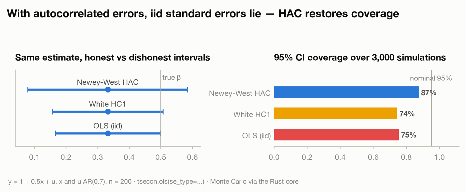
Robust standard errors: naive intervals lie, HAC restores coverage

The left panel is one representative sample where the naive 95% interval is so misleadingly tight it barely reaches the true \(\beta = 0.5\), while the honestly wider HAC interval covers it with room to spare. The right panel is the same comparison run 3,000 times — which brings us to the most useful habit this chapter can teach you.

⚠ Common mistake — Reaching for hc1 ("robust standard errors") on time series data. White-type corrections fix heteroskedasticity only; they assume independent errors and are just as overconfident as nonrobust when errors are serially correlated. In cross-sections, HC1 is the workhorse; in time series, the relevant rung is HAC or better.

A coverage experiment: Monte Carlo as a first-class tool¶

How do you know a standard error is honest? Theory gives asymptotic promises; a Monte Carlo experiment checks them at your sample size. The design pattern is always the same: simulate a world where you know the truth, apply the procedure many times, and count how often it succeeds. For confidence intervals the score is coverage: a nominal 95% interval should contain the truth in 95% of simulated samples. This is not just a textbook exercise — it is how econometricians evaluate procedures in published research, and tsecon treats it as a first-class workflow (the Rust core makes thousands of regressions per second routine).

The following experiment reproduces the right panel of the figure above, end to end:

n_mc, beta_true = 1000, 0.5
cover = {"nonrobust": 0, "hc1": 0, "hac": 0}

for rep in range(n_mc):
    y, x = simulate(seed=10_000 + rep)          # fresh world, known truth
    X = np.column_stack([np.ones(len(x)), x])
    for se in cover:
        r = tsecon.ols(y, X, se_type=se)
        b, s = r["params"][1], r["bse"][1]
        cover[se] += (b - 1.96 * s <= beta_true <= b + 1.96 * s)

print({k: v / n_mc for k, v in cover.items()})
# {'nonrobust': 0.742, 'hc1': 0.737, 'hac': 0.876}

Three lessons in three numbers. First, the naive interval covers 74% of the time while claiming 95% — in this design, roughly one in four "significant" findings at the 5% level would be false alarms. Second, HC1 does nothing, as promised. Third — and this is the honest part — Newey–West gets to 88%, not 95%. That remaining gap is the well-documented small-sample undercoverage of kernel HAC inference: \(\hat\Omega\) is itself noisy, and plugging it in as if it were the truth understates uncertainty. Closing that last gap is what the next section is about.

⚠ Common mistake — Seeding a Monte Carlo once at the top and letting all replications share one wandering RNG state. It works until you parallelize or re-order the loop, and then results silently change. Derive each replication's randomness from its own index (seed=10_000 + rep above): every replication becomes reproducible in isolation, and the experiment gives identical results in any execution order. The Philox section below shows why tsecon builds this contract into the core.

Fixed-b and EWC: the modern answer¶

Classical HAC theory makes an awkward assumption: as \(n \to \infty\) the bandwidth grows, but so slowly relative to \(n\) that \(\hat\Omega\) can be treated as if it were the true \(\Omega\). Under that fiction the t-statistic is compared to normal critical values. In real samples the fiction fails — \(\hat\Omega\) has substantial sampling error, the t-statistic has fatter tails than the normal, and coverage falls short, exactly as the experiment above showed.

Fixed-b asymptotics (Kiefer–Vogelsang 2005) drops the fiction. Treat the bandwidth as a fixed fraction \(b = S_n/n\) of the sample, and derive the actual limiting distribution of the t-statistic — which is no longer normal but depends on \(b\) and the kernel. Comparing the statistic to these wider, honest critical values corrects most of the size distortion. The insight reframes the problem: the bandwidth is not a nuisance to be estimated away but a choice of inference procedure, whose cost in power and benefit in size can be made explicit.

The most practical member of this family is the equal-weighted cosine (EWC) estimator, recommended as the default for applied work by Lazarus, Lewis, Stock, and Watson (2018). Project the (demeaned) series onto the first \(B\) cosine basis functions:

\[ \hat\Omega_{\text{EWC}} \;=\; \frac{1}{B}\sum_{j=1}^{B}\Lambda_j^2, \qquad \Lambda_j \;=\; \sqrt{\frac{2}{n}}\,\sum_{t=1}^{n}\cos\!\Bigl(\pi j\,\frac{t-\tfrac12}{n}\Bigr)\, x_t . \]

Each \(\Lambda_j\) is approximately an independent mean-zero normal with variance \(\Omega\), so \(\hat\Omega_{\text{EWC}}\) behaves like a \(\chi^2_B/B\) estimate of a variance — which means the resulting t-statistic follows, almost exactly, a Student-t distribution with \(B\) degrees of freedom. No simulated critical-value tables, no kernel arcana: pick \(B\), use \(t_B\) critical values. LLSW's size-power analysis recommends \(B = \lfloor 0.4\, n^{2/3}\rceil\) (about 22 at \(n=400\) — note how much wider this is than the rule-of-thumb's 5 lags, and how the small \(B\) tells you honestly that you have only ~22 effective degrees of freedom for estimating \(\Omega\)).

The EWC estimator and the LLSW default are already implemented and tested in tsecon's Rust core (ewc_lrv, ewc_default_b in the tsecon-hac crate) and land in Python with the Module 00 bindings.

Roadmap preview — this API lands with Module 00:

b  = tsecon.ewc_default_b(n)                 # LLSW 2018: round(0.4 * n^(2/3))
om = tsecon.ewc_lrv(scores, b=b)             # pair with t critical values, df = b

⚠ Common mistake — Using a wide bandwidth (or an EWC/fixed-b estimator) and then comparing the t-statistic to ±1.96. The entire point of fixed-b inference is that the critical values change with the smoothing choice: EWC with \(B = 22\) pairs with \(t_{22}\) critical values (±2.07 at 5%), not the normal's. Wide smoothing with normal critical values recreates the very overconfidence you were trying to fix.

The bootstrap, rebuilt for dependence¶

Sometimes there is no formula to fix. The statistic is a median, a ratio of coefficients, a turning-point date; the sample is short; the error distribution is visibly non-normal. The bootstrap's promise (Efron 1979) is to replace derivations with computation: resample your data with replacement many times, recompute the statistic each time, and use the spread of the recomputed values as the sampling distribution.

For time series the naive version of that promise is a trap. Resampling individual observations produces series in which today's value is a random draw from anywhere in the sample — the dependence structure is annihilated. And since positive dependence is exactly what inflates the variance of averages (section two), destroying it deflates the bootstrap's variance estimate. The iid bootstrap of a persistent series' mean concentrates around \(\gamma_0/n\) when the truth is \(\Omega/n\): for an AR(0.8), confidence intervals roughly three times too narrow — a precise, computational echo of the naive-standard-error mistake.

The repair is to resample blocks — contiguous chunks long enough to carry the dependence inside them:

Moving block (Künsch 1989): glue together randomly chosen length-\(\ell\) blocks until you have \(n\) observations.
Circular block (Politis–Romano 1992): the same, but the series wraps around end-to-start, so every observation appears in equally many blocks and the edge bias of the moving block disappears.
Stationary bootstrap (Politis–Romano 1994): block lengths are themselves random — geometric with mean \(1/p\) — which makes the resampled series stationary and the procedure less sensitive to any single block-length choice.

That leaves the block length, which plays exactly the role bandwidth played for kernels: too short breaks dependence, too long leaves too few distinct blocks. tsecon ships the Politis–White (2004) automatic selector (with the Patton–Politis–White 2009 correction) as a first-class function, not an exercise for the reader:

rng = np.random.default_rng(42)               # the AR(0.8) series from earlier
n = 400
e = rng.standard_normal(n)
y = np.empty(n); y[0] = 0.0
for t in range(1, n):
    y[t] = 0.8 * y[t - 1] + e[t]

opt = tsecon.optimal_block_length(y)          # {'stationary': 13.1, 'circular': 15.0}
p_star = 1.0 / opt["stationary"]              # restart probability: E[block] = 13.1

B = 2000
means = {"iid": np.empty(B), "block": np.empty(B)}
for b in range(B):
    i_iid = tsecon.bootstrap_indices(n, scheme="iid", seed=b)
    i_blk = tsecon.bootstrap_indices(n, scheme="stationary", seed=b, p=p_star)
    means["iid"][b]   = y[i_iid].mean()
    means["block"][b] = y[i_blk].mean()

target = np.sqrt(tsecon.long_run_variance(y, kernel="bartlett") / n)
print(means["iid"].std())     # ~0.076  -- far too confident
print(means["block"].std())   # ~0.167  -- brackets the truth
print(target)                 # ~0.147  -- the kernel benchmark

(bootstrap_indices returns index arrays rather than resampled data, so one call serves any statistic — apply the indices to y, to residuals, to whole rows of a multivariate panel. scheme="moving" and "circular" take block_length= instead of p=.)

The gallery figure runs this comparison at scale:

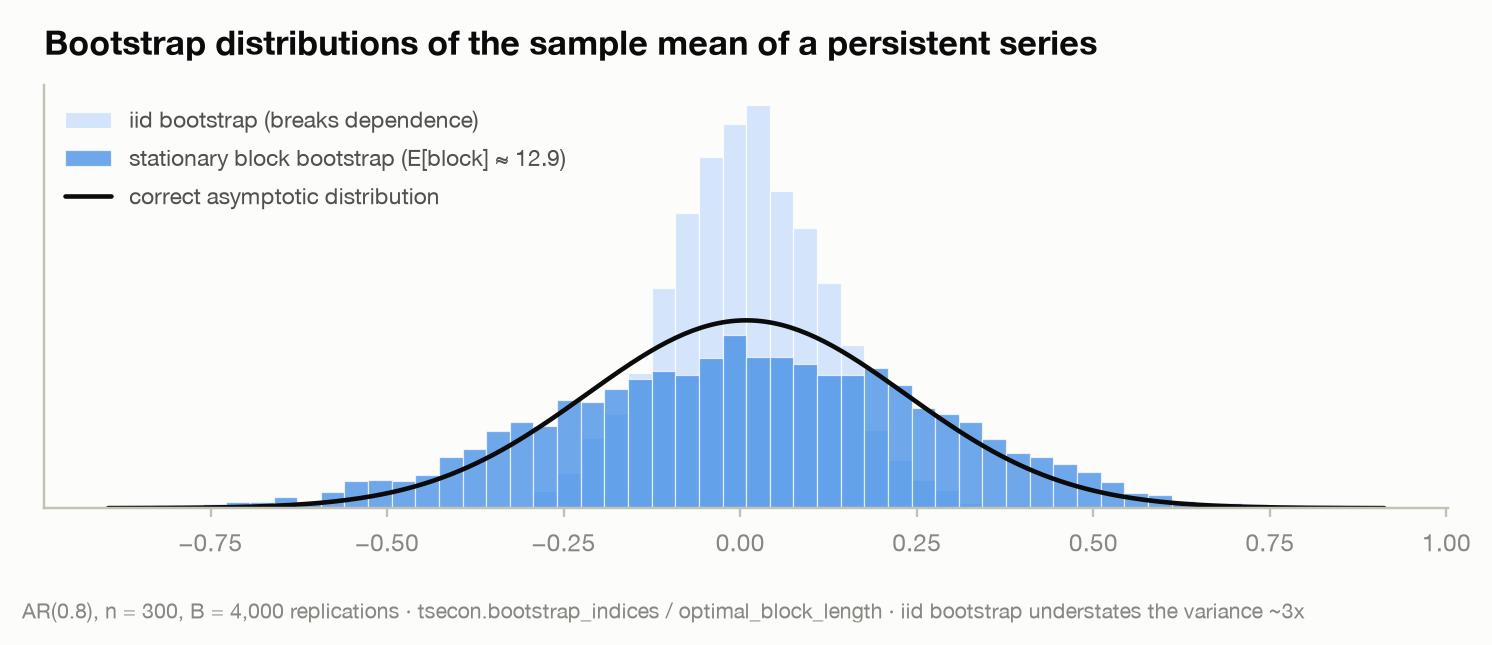
Bootstrap distributions: iid resampling is overconfident, block schemes are honest

The iid bootstrap distribution (light) is dramatically too narrow; the stationary block bootstrap (dark), with the automatically selected block length, lands on the correct asymptotic distribution (black curve). Note that the two honest methods — block bootstrap and kernel long-run variance — agree with each other, as they must: they are two estimators of the same \(\Omega\).

⚠ Common mistake — Bootstrapping residuals or observations of a time series iid because "the bootstrap is distribution-free." It is distribution-free, not dependence-free: the iid bootstrap's exchangeability assumption is precisely what stationary time series violate. If the data are dependent, the resampling scheme must preserve dependence — blocks, the sieve, or (for regression with independent-but-heteroskedastic errors) the wild bootstrap below.

The wild bootstrap for regressions¶

Regression brings its own resampling subtlety. Even with independent errors, resampling \((y_t, x_t)\) pairs changes the design matrix from replication to replication, and resampling residuals iid imposes homoskedasticity — it shuffles a large residual from a high-variance region onto a low-variance observation. The wild bootstrap (Wu 1986; Liu 1988; Mammen 1993) keeps every residual attached to its own observation and instead flips signs randomly:

\[ y_t^* \;=\; x_t'\hat\beta + w_t\,\hat u_t, \qquad \mathbb{E}[w_t] = 0,\quad \mathbb{E}[w_t^2] = 1 . \]

Each bootstrap sample has the same regressors and the same pattern of residual magnitudes — heteroskedasticity survives intact — while the random weights \(w_t\) generate sampling variation. The classic weight choices differ in their third moment: Rademacher weights (\(\pm 1\) with probability ½ each) impose symmetry and are the recommended default (Davidson–Flachaire 2008); Mammen's two-point weights match skewness to first order. Rademacher weights are a one-liner with tsecon's seeded uniforms:

rng = np.random.default_rng(7)
n = 120
x = rng.standard_normal(n)
u = (1.0 + 0.9 * np.abs(x)) * rng.standard_normal(n)   # heteroskedastic, independent
y = 1.0 + 0.5 * x + u
X = np.column_stack([np.ones(n), x])

r = tsecon.ols(y, X, se_type="hc1")
fitted = X @ r["params"]
resid  = y - fitted

B = 999
boot = np.empty(B)
for b in range(B):
    w = np.where(tsecon.philox_uniforms(seed=b, n=n) < 0.5, -1.0, 1.0)  # Rademacher
    y_star = fitted + w * resid
    boot[b] = tsecon.ols(y_star, X, se_type="hc1")["params"][1]

ci = np.percentile(boot - r["params"][1], [2.5, 97.5])
print(r["params"][1] - ci[1], r["params"][1] - ci[0])   # 95% percentile-t style interval

The Rust core ships the weight distributions as a dedicated primitive (WildWeights::Rademacher, Mammen, Normal in tsecon-bootstrap, with fixed per-draw stream costs so parallel replications stay aligned); the Python-level wild_bootstrap convenience lands with the Module 00 bindings.

⚠ Common mistake — Using the wild bootstrap to fix autocorrelation. Independent weights \(w_t\) destroy serial correlation in the residuals just as thoroughly as iid resampling does — the wild bootstrap is a heteroskedasticity tool. For serially correlated regression errors, use HAC/EWC standard errors, block-resample, or the dependent wild bootstrap (Shao 2010) on the roadmap, which draws the \(w_t\) as a smooth dependent process.

Reproducible randomness: Philox streams¶

Every method in the second half of this chapter consumes randomness by the megabyte, and modern hardware wants to consume it in parallel. That combination breaks naive RNG design. A conventional generator is a single sequential state machine: parallel workers either share it (race conditions, order-dependent results) or split it ad hoc (results change with the number of workers). Either way, "seed 42" stops meaning anything precise, and your published table becomes irreproducible the day you rerun it on a different machine.

tsecon's answer, inherited from the counter-based RNG literature (Salmon, Moraes, Dror, and Shaw 2011), is Philox: a generator that is a pure function rather than a state machine. Draw \(i\) of stream \(s\) under seed \(k\) is a fixed deterministic value — computed by encrypting the counter \(i\) with key \((k, s)\) — regardless of which thread asks for it, in what order, or how many threads exist. Reproducibility stops being a discipline you maintain and becomes an algebraic property:

u1 = tsecon.philox_uniforms(seed=42, n=1000)
u2 = tsecon.philox_uniforms(seed=42, n=1000)
assert (u1 == u2).all()                      # bit-identical, every time, every machine

g = np.random.Generator(np.random.Philox(42))
assert (u1 == g.random(1000)).all()          # bit-identical to NumPy's Philox

The second assertion is a design contract, not a coincidence: tsecon's Rust implementation reproduces NumPy's Philox bit for bit, with golden vectors locked in CI, so simulation studies validated against NumPy transfer exactly.

The bootstrap loops above already used the idiom this enables: replication \(b\) draws from its own stream (seed=b), so each replication's randomness is a pure function of its index. The Rust core generalizes this into the par_replicate engine — every bootstrap and Monte Carlo in the library derives replication \(b\)'s stream from (seed, \(b\)) and runs replications across threads via rayon — which yields the library's headline guarantee: the same seed produces bit-identical results at 1, 4, or 16 threads. No mainstream econometrics package makes that promise; it is why a tsecon bootstrap table in a paper is reproducible from the seed alone, forever.

⚠ Common mistake — Believing reproducibility claims transfer across everything. Thread-count invariance and same-platform bit-identity are guaranteed; bit-identity across operating systems and CPU generations is not (math-library and FMA differences at the last bit), and tsecon's documentation says so rather than promising the impossible. Record the platform alongside the seed for exact replication.

Interrogating the model: specification and stability tests¶

Everything so far has repaired the variance of an estimate while quietly trusting the model. The sandwich formula, HAC, EWC, the block bootstrap — every one of them takes the regression \(y_t = x_t'\beta + u_t\) as correctly specified and stationary, and fixes only how uncertain \(\hat\beta\) is. But a standard error, however robust, is a statement about sampling variability around a target. If the target is wrong — the conditional mean is not linear, the variance is not constant, the coefficients drifted mid-sample — then no denominator saves you. You would be reporting a beautifully calibrated interval around the wrong number. Before you trust an inference, you have to interrogate the assumptions that produced it.

Three of those assumptions are checkable, and each has a test whose null is "the assumption holds." Read a rejection not as a repair but as a redirection — it tells you which maintained assumption failed and therefore which fix to reach for.

Constant error variance. heteroskedasticity_test regresses the squared residuals on functions of the design. White (1980) is the omnibus version — residuals on the columns, their squares, and cross-products — with power against general heteroskedasticity; Koenker's studentised Breusch–Pagan regresses on the design alone, a focused, higher-power test when the variance is linear in a regressor. Null: homoskedasticity. A rejection means your nonrobust standard errors are wrong — climb the ladder to hc1 (cross-section) or hac/EWC (time series). It is a cue to change the denominator, not to abandon the model.
Correct functional form. reset_test (Ramsey 1969) refits with low-order powers of the fitted values, \(\hat y^2, \hat y^3\), appended to the design and \(F\)-tests whether they belong. The fitted value is a parsimonious index standing in for whatever nonlinearity you left out. Null: the linear mean is correct. A rejection means you have the form wrong — and here robust standard errors do not help, because the problem is \(\beta\) itself, not \(\mathrm{Var}(\hat\beta)\).
Stable coefficients. chow_test (Chow 1960) splits at a break date you know — a policy change, a crisis onset — and \(F\)-tests whether the two regimes share one \(\beta\). cusum_test (Brown–Durbin–Evans 1975) scans the whole sample when you do not know the date: it accumulates recursive residuals into a path that stays inside a pair of boundary lines under stability and drifts out through them when \(\beta\) moves. Null (both): the relationship held still. A rejection means it moved — reach for a split-sample fit, interactions with a regime dummy, or a time-varying model.

One input contract binds all four, and it is the single most common way to trip over them: the design must carry an explicit intercept column of ones. These are auxiliary-regression LM and \(F\) tests whose statistics are only valid when the auxiliary design has an intercept, so tsecon refuses to guess — a design without a constant raises MissingConstant rather than silently adding one. There is also an ordering discipline: run reset_test before heteroskedasticity_test, because a misspecified mean leaves structure in the residuals that a variance test will misread as heteroskedasticity. Fix the form first, then ask about the variance.

The cleanest way to see what each test is for is to break one assumption at a time and watch exactly one test light up:

import numpy as np, tsecon

n = 240
t = np.arange(n)

def battery(y, X):
    reset = tsecon.reset_test(y, X, max_power=3)["pvalue"]
    white = tsecon.heteroskedasticity_test(y, X, test="white")["pvalue"]
    chow  = tsecon.chow_test(y, X, split=160)["pvalue"]
    cus   = tsecon.cusum_test(y, X)
    breach = bool(np.any(cus["path"] > cus["bound_upper"]) or
                  np.any(cus["path"] < cus["bound_lower"]))
    return reset, white, chow, breach

rng = np.random.default_rng(0)
x1 = rng.uniform(1.0, 4.0, size=n)
X = np.column_stack([np.ones(n), x1])                       # constant column -- required

scenarios = {
    "well-specified": 1.0 + 0.5 * x1 + rng.normal(size=n),
    "omitted x1^2":   1.0 + 0.5 * x1 + 0.4 * x1**2 + rng.normal(size=n),
    "variance ~ x1":  1.0 + 0.5 * x1 + x1 * rng.normal(size=n),
    "break at t=160": 1.0 + 0.5 * x1 + rng.normal(size=n) + 2.0 * (t > 160),
}

print(f"{'scenario':>16} | {'RESET':>7} {'White':>7} {'Chow':>7} | CUSUM")
print("-" * 56)
for label, y in scenarios.items():
    reset, white, chow, breach = battery(y, X)
    print(f"{label:>16} | {reset:7.4f} {white:7.4f} {chow:7.4f} | {breach}")

#         scenario |   RESET   White    Chow | CUSUM
# --------------------------------------------------------
#   well-specified |  0.8954  0.8057  0.2541 | False
#     omitted x1^2 |  0.0000  0.2877  0.7850 | False
#    variance ~ x1 |  0.0146  0.0000  0.5660 | False
#   break at t=160 |  0.2342  0.7541  0.0000 | True

The near-diagonal pattern is the whole lesson. The well-specified row is quiet everywhere. Omitting the true \(x_1^2\) term lights up RESET alone; a variance that scales with \(x_1\) lights up White decisively (with a small RESET leak — a reminder that these symptoms are not perfectly orthogonal, and why RESET goes first); a mid-sample intercept jump lights up Chow and pushes the CUSUM path across its band, precisely because Chow was handed the right date while CUSUM found the instability on its own. Notice that CUSUM returns a boolean-from-a-path, not a p-value: the model card documents its four keys (path, bound_upper, bound_lower, sigma) and the per-test argument contracts.

⚠ Common mistake — Handing these tests a design with no constant column ("the intercept is implied"). It is not — heteroskedasticity_test, reset_test, chow_test, and cusum_test all raise MissingConstant, by design, because their auxiliary statistics are only valid with an explicit intercept. Always pass X = np.column_stack([np.ones(n), ...]). And read a rejection as a redirection, never as a death sentence: heteroskedasticity → robust standard errors, RESET → a richer functional form, Chow/CUSUM → a model whose coefficients are allowed to move.

When the predictor is persistent: predictive regressions and IVX¶

There is one setting where even a correctly specified, stable regression yields a t-test you should not believe — and it is common enough in finance and macro to deserve its own section. You want to know whether a slow-moving variable predicts next period's return: regress \(r_{t+1}\) on a dividend yield, a term spread, a valuation ratio. Two features of that regression conspire against you. The predictor is persistent — its autoregressive root sits near one, the near-unit-root territory of the ADF discussion in Chapter 2 — and its innovation is correlated with the return it is meant to forecast (endogeneity). That combination is the Stambaugh (1999) setting, and in it OLS misbehaves twice:

\[ r_{t+1} = \alpha + \beta\, x_t + u_{t+1}, \qquad x_t = \rho\, x_{t-1} + e_t, \qquad \rho \approx 1,\ \ \mathrm{Corr}(u_{t+1}, e_t) \neq 0 . \]

First, the slope \(\hat\beta\) is biased in finite samples — the least-squares root bias in \(\hat\rho\) (Kendall 1954) leaks into \(\hat\beta\) through the endogeneity. Second, and worse for inference, the OLS t-statistic over-rejects a true "no predictability" null, and the distortion grows as \(\rho \to 1\). The near-integrated regressor breaks the standard normal approximation for the t-statistic, so comparing it to \(\pm 1.96\) manufactures significance that is not there. This is not something HAC fixes: HAC repairs serial correlation in the errors, but here the errors can be perfectly clean — the problem is the regressor's near-unit-root persistence combined with endogeneity, a different disease entirely.

The cure is IVX (Kostakis, Magdalinos & Stamatogiannis 2015), which instruments the persistent predictor with a self-generated mildly integrated process \(z_t\) — more persistent than any stationary variable but strictly less than a unit root. That instrument is persistent enough to be relevant yet just stationary enough to deliver a well-behaved limit, so the resulting Wald test of \(H_0:\beta = 0\) is asymptotically \(\chi^2\) uniformly over the predictor's persistence — whether \(x_t\) is stationary, near-integrated, or an exact unit root. predictive_regression returns three views of the same regression in one call: the misleading ols benchmark, the stambaugh bias-corrected point estimate, and the ivx Wald test you should actually report.

import numpy as np, tsecon

# One draw: a near-unit-root predictor, endogenous innovation, TRUE slope = 0.
rng = np.random.default_rng(0)
n, rho, corr = 300, 0.99, -0.9
e = rng.standard_normal(n)
x = np.zeros(n)
for t in range(1, n):
    x[t] = rho * x[t - 1] + e[t]
u = corr * e + np.sqrt(1 - corr**2) * rng.standard_normal(n)
r = u                                              # beta = 0: nothing to predict

fit = tsecon.predictive_regression(r, x)
print(f"OLS  : beta={fit['ols']['beta']:+.4f}  t={fit['ols']['tstat']:+.2f}")
print(f"IVX  : beta={fit['ivx']['beta_ivx']:+.4f}  Wald={fit['ivx']['wald']:.2f}  "
      f"p={fit['ivx']['pvalue']:.3f}")

# OLS  : beta=+0.0123  t=+1.06
# IVX  : beta=+0.0108  Wald=0.85  p=0.358

A single draw only illustrates the machinery; the claim is about repeated sampling, and it is exactly a size claim of the kind the coverage experiment above taught you to check. Simulate a true null (\(\beta = 0\)) across a ladder of persistence and count how often each test rejects at the nominal 5%:

chi2_95, z_95 = 3.841, 1.96
corr = -0.9
print(f"{'rho':>6} | {'OLS t-test':>11} | {'IVX Wald':>9}")
print("-" * 34)
for rho in [0.90, 0.95, 0.99, 1.00]:
    rej_ols = rej_ivx = 0
    reps = 1000
    for rep in range(reps):
        g = np.random.default_rng(int(rho * 100) * 10_000 + rep)  # per-replication stream
        e = g.standard_normal(300)
        x = np.zeros(300)
        for t in range(1, 300):
            x[t] = rho * x[t - 1] + e[t]
        u = corr * e + np.sqrt(1 - corr**2) * g.standard_normal(300)
        f = tsecon.predictive_regression(u, x)          # r = u, true beta = 0
        rej_ols += abs(f["ols"]["tstat"]) > z_95
        rej_ivx += f["ivx"]["wald"] > chi2_95
    print(f"{rho:6.2f} | {rej_ols/reps:11.3f} | {rej_ivx/reps:9.3f}")

#    rho |  OLS t-test |  IVX Wald
# ----------------------------------
#   0.90 |       0.058 |     0.055
#   0.95 |       0.065 |     0.051
#   0.99 |       0.131 |     0.048
#   1.00 |       0.238 |     0.046

Read the OLS column top to bottom: a test that is meant to reject 5% of the time creeps to 13% at \(\rho = 0.99\) and to 24% at an exact unit root — roughly one "significant predictor" in four is a phantom, and it is precisely the persistent predictors (dividend yields, valuation ratios) where the distortion is worst. The IVX column holds its size across the entire ladder, including \(\rho = 1\). The library's Monte Carlo suite runs this at larger scale and pins the exact-unit-root numbers at 27.8% for OLS versus 5.3% for IVX — over five times the nominal rate, dissolved. For a panel of competing predictors, ivx_test gives the same uniform-size guarantee for a single joint Wald test; both functions and the Stambaugh view are documented in the predictive-regressions model card.

⚠ Common mistake — Reaching for HAC or Newey–West standard errors to rescue a predictive regression on a persistent predictor. HAC corrects serial correlation in the residuals; the Stambaugh problem is near-unit-root persistence in the regressor combined with endogeneity, which HAC leaves untouched — the over-rejection survives. And do not read IVX's honesty as pessimism: it controls size, not power, so a large p-value near a unit root means "no evidence of predictability," not "predictability disproven."

Beyond the mean: quantile regression¶

Everything in this chapter so far has been about one target: the conditional mean, and how uncertain its estimate is. But "how does \(x\) move the average of \(y\)" is only one question you can ask a conditional distribution, and for many economic problems it is the wrong one. A risk manager cares about the 5th percentile of returns, not the mean; a labor economist asking whether education compresses or stretches the wage distribution needs the whole ladder of quantiles; the growth-at-risk workflow in the forecasting chapter is built on nothing else. Quantile regression (Koenker and Bassett, 1978) makes any conditional quantile a regression target — same design matrix, different loss.

The trick is the check loss (you will meet it again as the pinball loss when the forecasting chapter scores quantile forecasts):

\[ \rho_\tau(u) \;=\; u\,\bigl(\tau - \mathbf{1}\{u < 0\}\bigr), \]

an asymmetrically tilted absolute value: positive residuals cost \(\tau |u|\), negative ones cost \((1-\tau)|u|\). Minimizing \(\sum_t \rho_\tau(y_t - x_t'\beta)\) over \(\beta\) estimates the conditional \(\tau\)-quantile, for exactly the reason the median minimizes absolute error: the asymmetry is calibrated so the optimal fit leaves a fraction \(\tau\) of the observations below it. Set \(\tau = 0.5\) and you have median regression; sweep \(\tau\) across \((0,1)\) and you trace out how the entire shape of the conditional distribution moves with \(x\).

When does this tell you something OLS cannot? There is a sharp null case: if the model is a pure location shift — \(y = x'\beta + u\) with iid errors — then every quantile's slope equals the OLS slope, and the quantile fits differ only in their intercepts. Quantile regression earns its keep exactly when that fails: under heteroskedasticity (the spread of \(y\) depends on \(x\), so upper and lower quantile slopes fan apart) or asymmetry (a covariate that lengthens one tail only). Both are the norm, not the exception, in economic data.

Inference needs one more idea. The asymptotic variance of a quantile estimator has a sandwich form whose meat involves the sparsity — one over the density of the errors at the quantile being estimated. Intuition: where data are dense, the quantile is pinned down precisely; in a sparse tail, it wobbles. The density must itself be estimated, and quantile_regression does it the standard way (Powell, 1991): a kernel estimate of the density at the fitted quantile, Epanechnikov kernel, Hall-Sheather (1988) bandwidth — the same estimator statsmodels' QuantReg reports, matched at 1e-6 in the test suite, with the IRLS coefficients matched likewise.

Watch the slopes fan apart on a location-scale model where the spread of \(y\) grows with \(x\):

rng = np.random.default_rng(21)
n = 600
x = rng.uniform(0.0, 4.0, n)
u = rng.standard_normal(n)
y = 1.0 + 0.5 * x + (0.4 + 0.45 * x) * u        # true tau-slope: 0.5 + 0.45 * z_tau
X = np.column_stack([np.ones(n), x])            # include your own constant, as always

qr = tsecon.quantile_regression(y, X, taus=[0.10, 0.50, 0.90])
for i, tau in enumerate(qr["taus"]):
    b, s, tv = qr["params"][i], qr["bse"][i], qr["tvalues"][i]
    print(f"tau={tau}: slope {b[1]:+.3f}  (se {s[1]:.3f}, t {tv[1]:+.1f})")

# tau=0.1: slope -0.092  (se 0.058, t -1.6)     true: -0.077
# tau=0.5: slope +0.574  (se 0.048, t +12.0)    true: +0.500
# tau=0.9: slope +1.185  (se 0.064, t +18.7)    true: +1.077

r = tsecon.ols(y, X, se_type="hc1")
print(round(r["params"][1], 3))                  # 0.541 — the mean slope, one number for three stories

OLS reports a single slope of 0.54 and, with its HC1 standard error, reports it honestly — but it is an honest answer to a question that averages away the phenomenon. The quantile ladder shows what is actually happening: at the 10th percentile the slope is statistically indistinguishable from zero, at the median it is 0.57, at the 90th it is 1.19 — all three within two standard errors of their true values (\(0.5 + 0.45\,z_\tau\)). The relationship lives in the upper tail and vanishes in the lower one, and no amount of robust-standard-error machinery on the mean regression could have said so. The result dict also carries per-tau bandwidth and sparsity (report them, for the same reproducibility reason you report a HAC bandwidth) and a single converged flag over all taus. Full contract and validation: the quantile model card.

Two pointers for where this machinery goes next. Dynamic responses of quantiles to shocks — how a financial shock moves the left tail of future GDP growth — are quantile local projections, tsecon.quantile_lp (Chapter 9); the full policy-institution workflow around them is growth-at-risk, tsecon.growth_at_risk (Chapter 5).

⚠ Common mistake — Fitting quantiles one \(\tau\) at a time and treating the fits as a coherent distribution. Each \(\tau\) is estimated separately, so nothing forces the fitted 90th percentile to sit above the fitted 50th at every \(x\) — quantile crossing is a finite-sample fact of life, worst in small samples and at extreme taus. If you need a valid distribution (fan charts, density evaluation), sort the fitted quantiles at each observation — the Chernozhukov–Fernández-Val–Galichon rearrangement, which growth_at_risk applies for you and flags via crossing. A second trap: the Powell sandwich here assumes independent errors — it is the quantile analogue of HC, not HAC. For strongly autocorrelated data, treat the reported bse as a lower bound and lean on the moving-block bootstrap from this chapter.

The frontier¶

Heteroskedasticity-and-autocorrelation-robust ("HAR") inference is an unusually live corner of econometric theory, and its modern consensus is recent. The state of the art:

Size-power frontiers. Lazarus, Lewis, Stock, and Watson (2018) turned decades of bandwidth folklore into explicit recommendations (EWC, \(B = 0.4\,n^{2/3}\), \(t_B\) critical values); Lazarus, Lewis, and Stock (2021) proved formal bounds on the trade-off between size distortion and power loss, showing the LLSW rule is near the frontier — there is provably no free lunch left in bandwidth choice. Sun (2014) unifies the fixed-b and orthonormal-series ("fixed-smoothing") viewpoints. Müller (2014) shows that for strongly autocorrelated series all standard HAR procedures remain fragile, proposing inference tailored to near-unit-root persistence — the honest frontier: no known procedure is uniformly reliable as persistence approaches a unit root.
Bootstrap refinements. The dependent wild bootstrap (Shao 2010) and tapered block bootstrap (Paparoditis–Politis 2001) improve on plain blocks; the sieve bootstrap resamples innovations of a fitted AR approximation; Hansen's (1999) grid bootstrap remains the canonical fix for confidence intervals on autoregressive roots near unity, where all first-order asymptotics fail. Higher-order theory for when block bootstraps beat asymptotics is comprehensively treated in Lahiri (2003).
Reproducible computation. Counter-based RNGs have made deterministic parallel simulation cheap (Salmon et al. 2011), but journal replication standards still rarely demand thread-count-invariant results; libraries that guarantee them by construction are ahead of the norms.

On tsecon's roadmap (Module 00), this chapter's machinery deepens in three directions: the full HAC policy layer (Andrews and Newey–West automatic bandwidths, prewhitening, fixed-b critical values, EWC as the library-wide default policy following LLSW); the extended resampling schemes (sieve, dependent wild, tapered block, subsampling with rate estimation, and the Hansen grid bootstrap, validated against the published REStat intervals); and the par_replicate engine surfacing in Python so user-written Monte Carlo studies inherit the thread-invariance guarantee. Open problems the roadmap is honest about: no automatic bandwidth is reliable under near-unit-root persistence, and small-\(n\) HAR inference for multivariate hypotheses (joint F-tests) is measurably worse than the scalar case the theory is tuned for.

Which method when¶

Situation	Reach for	Because
Standard error of the mean (or any average) of a stationary series	`long_run_variance(y) / n`, square root	The naive \(s/\sqrt{n}\) ignores every cross-covariance; \(\Omega\) is the honest variance
Time series regression, routine inference	`ols(y, X, se_type="hac")`	Coefficients stay OLS; the variance accounts for autocorrelation and heteroskedasticity
Cross-section or independent errors, unequal variances	`ols(y, X, se_type="hc1")`	White's fix is enough when there is no serial correlation; HAC would waste power
Persistent errors, sample not huge, size matters	EWC with \(t_B\) critical values (bindings landing; Rust core today)	Kernel HAC with normal critical values undercovers; fixed-b/EWC prices in the noise of \(\hat\Omega\)
Nonstandard statistic (median, ratio, custom estimator) on dependent data	`optimal_block_length` + `bootstrap_indices(scheme="stationary")`	No formula needed; blocks preserve the dependence that drives the true sampling variance
Regression, independent but heteroskedastic errors, small sample	Wild bootstrap (Rademacher weights via `philox_uniforms`)	Keeps each residual's variance attached to its observation; refines on HC asymptotics
Serially correlated and heteroskedastic regression errors, asymptotics dubious	Block bootstrap of the regression, or HAC/EWC	Wild bootstrap alone breaks the serial correlation; blocks or kernels respect it
Evaluating a procedure (does my CI cover? does my test have size 5%?)	A seeded Monte Carlo with per-replication streams (`seed=base+rep`)	Coverage is checkable, not guessable — and per-index streams make the experiment exactly reproducible
Before trusting any regression inference: is the model even right?	`reset_test` (form), `heteroskedasticity_test` (variance), `chow_test`/`cusum_test` (stability)	A robust standard error is honest only if the mean, variance, and coefficients are what you assumed; test that first
Predicting a return with a persistent, endogenous predictor	`predictive_regression` / `ivx_test` (report the IVX Wald)	The OLS t-test over-rejects near a unit root; IVX keeps its size uniformly over the predictor's persistence
The question is about a tail or the distribution's shape, not the mean	`quantile_regression`	Check-loss estimation targets any conditional quantile; slopes fan apart under heteroskedasticity or asymmetry that OLS averages away
AR root near one, confidence interval for persistence	Grid bootstrap (roadmap)	Standard asymptotics and standard bootstraps are both invalid near the unit root

What tsecon implements today¶

Available now in Python (import tsecon):

tsecon.ols(y, X, se_type=..., maxlags=..., use_correction=...) — OLS with the full ladder: "nonrobust", "hc0", "hc1", "hac" (Bartlett kernel; maxlags=None applies the Newey–West rule of thumb). Matches statsmodels cov_type="HAC" at 1e-10. X is used as-is — add your own constant column.
tsecon.long_run_variance(x, kernel=..., bandwidth=...) — kernel LRV of a series (demeaned internally); kernels "bartlett"/"newey-west", "parzen", "qs", "truncated".
tsecon.bootstrap_indices(n, scheme=..., seed=..., block_length=..., p=...) — resampling indices for "iid", "moving", "circular" (pass block_length), and "stationary" (pass p; expected block length \(1/p\)). Same seed, same indices, always.
tsecon.optimal_block_length(y) — Politis–White (2004) automatic block lengths with the Patton–Politis–White (2009) correction, for the stationary and circular schemes.
tsecon.philox_uniforms(seed, n) — seeded uniform draws, bit-compatible with numpy.random.Philox.
tsecon.heteroskedasticity_test(y, X, test=...), tsecon.reset_test(y, X, max_power=...), tsecon.chow_test(y, X, split=...), tsecon.cusum_test(y, X) — the specification-and-stability battery (White / Koenker–Breusch–Pagan, Ramsey RESET, Chow, Brown–Durbin–Evans CUSUM). X must include an explicit constant column. See the specification-tests model card.
tsecon.predictive_regression(r, x) and tsecon.ivx_test(r, xs) — OLS / Stambaugh / IVX views of a predictive regression and the joint IVX Wald test, with correct size uniformly over a persistent predictor's root. See the predictive-regressions model card.
tsecon.quantile_regression(y, x, taus=...) — IRLS check-loss coefficients with Powell kernel-sandwich standard errors (Epanechnikov kernel, Hall-Sheather bandwidth); per-tau params, bse, tvalues, bandwidth, sparsity, plus converged. statsmodels-QuantReg-validated at 1e-6; include your own constant column. See the quantile model card.

Built in Rust, awaiting Python bindings (in tsecon-hac and tsecon-bootstrap):

EWC long-run variance and the LLSW default degrees of freedom (ewc_lrv, ewc_default_b).
Andrews (1991) AR(1) plug-in and Newey–West (1994) automatic bandwidths (andrews_bandwidth_ar1, newey_west_bandwidth).
AR(1)-prewhitened LRV, Andrews–Monahan style (lrv_prewhitened_ar1).
Wild-bootstrap weight generators — Rademacher, Mammen, normal — with fixed per-draw stream costs (WildWeights).
The sequential and parallel replication engine with per-replication substreams (replicate, par_replicate) — thread-count-invariant by construction.

Roadmap (docs/roadmap/00-architecture.md): fixed-b critical values (Kiefer–Vogelsang), the library-wide LLSW-based HAC default policy, sieve bootstrap, dependent wild bootstrap (Shao 2010), tapered block bootstrap (Paparoditis–Politis 2001), subsampling with convergence-rate estimation, the Hansen (1999) grid bootstrap for near-unit-root AR inference, and fast double/nested bootstrap.