Chapter 4 — Univariate Models: AR to State Space
Part of The tsecon Guide to Time Series Econometrics. Chapters mirror the library's modules; code runs against the current Python API unless marked otherwise.
Prerequisites: the stationarity toolkit (ADF, KPSS, differencing) from the earlier chapters, plus OLS and maximum likelihood at first-econometrics-course level.
You will learn:
- how the AR → MA → ARMA → ARIMA → SARIMA ladder assembles one model family from two simple parts
- why conditional sum of squares (CSS) and exact maximum likelihood give different answers in small samples, and which to trust
- how AIC/BIC and auto-ARIMA choose model orders — and the classic ways automatic selection goes wrong
- what the state-space form and the Kalman filter actually do, and why missing data costs them nothing
- when to leave the linear world: regime switching, thresholds, and (at the frontier) long memory
The idea
Suppose you need to forecast next quarter's GDP growth. You have exactly one thing: the history of GDP growth itself. No structural model, no other variables. Can you do anything useful?
Almost always yes, because economic time series have momentum. A quarter of strong growth tends to be followed by another decent quarter; a spike in inflation fades over several months rather than vanishing overnight. The whole univariate modeling enterprise is a machine for measuring that momentum and projecting it forward.
There are two natural ways to describe momentum, and they turn out to be the two atoms everything in this chapter is built from:
- The past of the series predicts its future. "GDP growth was above average last quarter, so it will probably be above average this quarter, just less so." This is autoregression — literally, a regression of the series on itself.
- Past surprises linger. "The oil shock three months ago is still working its way into prices." Here the series is a weighted memory of recent random shocks. This is a moving average of shocks.
Everything else is assembly. Combine the two and you get ARMA. Notice that some series (the level of GDP, prices, the money stock) drift without ever returning to a mean, so you model their changes instead — that is the "I" (integrated) in ARIMA. Notice that December looks like last December, and you get seasonal ARIMA. Notice that you'd rather think in terms of an unobserved "true" level being measured with noise — like trying to read the economy's underlying state through statistical fog — and you arrive at the state-space form and the Kalman filter, which quietly turns out to be the engine that estimates all the other models too.
Picture the simplest case as a thermostat-controlled room with a drafty window. The temperature (the series) keeps getting knocked around by gusts (shocks), but the thermostat pulls it back toward the set point (the mean). How hard it pulls is the autoregressive coefficient. If the thermostat is strong, disturbances die out quickly and the series hugs its mean; if it is weak, the room stays cold for a long time after each gust; if it is absent entirely, the temperature wanders wherever the gusts push it — a random walk, and the boundary of the stationary world. This chapter is about measuring the thermostat.
Autoregression: momentum you can regress on
A practitioner cares about AR models because they are the cheapest credible answer to "how persistent is this series?" — the question behind inflation half-lives, output-gap dynamics, and nearly every benchmark forecast.
An AR(p) (autoregression of order p) says today's value is a linear function of the last \(p\) values plus a fresh shock:
where \(c\) is an intercept, the \(\phi_j\) are the autoregressive coefficients, and \(\varepsilon_t\) (the innovation) is the part of \(y_t\) that nothing in the past could have predicted.
Stationarity — the requirement that the series keeps returning to a fixed mean with stable variance — puts a condition on the coefficients. For an AR(1), \(y_t = c + \phi y_{t-1} + \varepsilon_t\), the condition is simply \(|\phi| < 1\): each period the deviation from the mean shrinks by the factor \(\phi\). At \(\phi = 1\) the thermostat is gone and you have a random walk. For general \(p\), write the model with the lag polynomial \(\phi(L) = 1 - \phi_1 L - \cdots - \phi_p L^p\) (where \(L\) is the lag operator, \(L y_t = y_{t-1}\)); stationarity requires every root \(z\) of \(\phi(z) = 0\) to lie outside the unit circle. When it holds, the AR(1) mean is \(\mu = c / (1 - \phi)\) — a formula worth memorizing, because the intercept of an AR model is not its mean.
The Yule-Walker equations are the moment-based route to estimation, and the intuition is worth having even if you always use maximum likelihood. Multiply the AR equation by \(y_{t-k}\), take expectations, and divide by the variance: the autocorrelations \(\rho_k\) must satisfy
The model's own recursion governs its correlation structure. Stack the first \(p\) of these equations, plug in sample autocorrelations, and solve for the \(\phi_j\): that is Yule-Walker estimation. It also explains the two identification fingerprints of an AR(p): the ACF decays geometrically (the recursion never lets it stop dead), while the partial autocorrelation function (PACF) — the correlation between \(y_t\) and \(y_{t-k}\) after controlling for everything in between — cuts off sharply after lag \(p\).
You can see both fingerprints, and evaluate the exact likelihood, with today's API:
import numpy as np
import tsecon

rng = np.random.default_rng(42)
n = 400
phi1, phi2 = 1.3, -0.4          # a stationary AR(2)
y = np.zeros(n)
eps = rng.standard_normal(n)
for t in range(2, n):
    y[t] = phi1 * y[t-1] + phi2 * y[t-2] + eps[t]

r = tsecon.acf(y, nlags=24)      # dict: acf, bartlett_se
p = tsecon.pacf(y, nlags=24)     # Yule-Walker ("yw") or "ols"

# exact Gaussian log-likelihood at candidate parameters
tsecon.ar_loglik(y, [1.3, -0.4], sigma2=1.0)   # the truth
tsecon.ar_loglik(y, [0.9, 0.0], sigma2=1.0)    # a worse model: lower loglik

# a one-dimensional exact MLE by brute force, to see the machinery move.
# With phi2 = -0.4 fixed, stationarity requires phi1 + phi2 < 1, i.e.
# phi1 < 1.4 — the admissible region is a triangle, not a box, and
# ar_loglik refuses to evaluate outside it.
grid = np.linspace(1.0, 1.39, 79)
ll = [tsecon.ar_loglik(y, [g, -0.4], sigma2=1.0) for g in grid]
phi1_hat = grid[np.argmax(ll)]                 # lands near 1.3
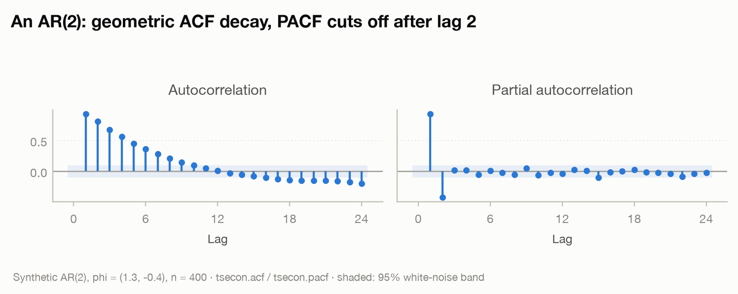
The figure is this exact process: smooth ACF decay, two PACF spikes, then nothing — you read "AR(2)" straight off the plot. ar_loglik is not a toy: it evaluates the exact Gaussian likelihood through the state-space form with a stationary initial distribution, the same kernel a full ARIMA fit maximizes (more on this below).
⚠ Common mistake. Fitting an AR model to a series you have not checked for stationarity. If the true process has a unit root, the fitted \(\phi\) will hug 1, forecasts will be garbage at long horizons, and standard errors are invalid. Run
tsecon.check_stationarity(y)first. A subtler trap: Yule-Walker estimates are mechanically biased toward stationarity near the unit circle (R'sar()default suffers from this), so near-unit-root persistence is systematically understated — one reason exact MLE is the default worth having.
Moving averages and the ARMA compromise
Why would anyone model a series as a function of unobservable shocks? Because some economic quantities genuinely have finite memory of surprises. A one-off measurement quirk in this month's CPI affects the next release or two of the inflation rate and then is gone completely. An AR model cannot produce that pattern — its shocks decay geometrically but never fully vanish.
An MA(q) (moving average of order q) writes the series as a weighted sum of the last \(q+1\) innovations:
An MA(q) is always stationary (it is a finite sum of white noise), and its ACF is exactly zero beyond lag \(q\) — the mirror image of the AR fingerprint. The condition that matters instead is invertibility: the roots of \(\theta(z) = 1 + \theta_1 z + \cdots + \theta_q z^q\) must lie outside the unit circle. The reason is identification, not stability: an MA(1) with coefficient \(\theta\) and one with \(1/\theta\) produce identical autocorrelations, so the data cannot tell them apart. The invertible representation is the one in which the shocks can be recovered from the observed history — the one where \(\varepsilon_t\) means what you think it means.
Why combine the two? Parsimony. The Wold decomposition theorem (Wold, 1938) says every covariance-stationary process is an MA(\(\infty\)) — an infinite weighted sum of past shocks. You cannot estimate infinitely many weights, but a ratio of two short polynomials can approximate a long one remarkably well, exactly as a rational function approximates a complicated curve better than a polynomial of the same total degree. That is the ARMA(p,q):
An ARMA(1,1) with two dynamic parameters often fits what would take an AR(5) or an MA(8) — fewer parameters, tighter estimates, better forecasts. This trade is the heart of the Box-Jenkins methodology (Box and Jenkins, 1970): identify a small model from the ACF/PACF, estimate it, check the residuals, and only grow the model if the residuals demand it.
The residual check is available today, and it has a degrees-of-freedom subtlety worth internalizing now:
# fit an ARMA(2,1) to the AR(2) series from the first block, then ask
# whether its one-step residuals still carry structure
fit   = tsecon.arima_fit(y, p=2, d=0, q=1, constant=True)
resid = fit["residuals"]
lb = tsecon.ljung_box(resid, nlags=10)   # dict: lags, lb_stat, lb_pvalue, ...
⚠ Common mistake. Two, actually. First: the Ljung-Box test on model residuals must have its degrees of freedom reduced by the number of fitted ARMA parameters — comparing the statistic at lag 10 to a \(\chi^2_{10}\) after fitting an ARMA(2,1) overstates the p-value; use \(\chi^2_{10-3}\). Second: overfitting ARMA orders creates near-canceling roots — an ARMA(2,2) fit to ARMA(1,1) data puts an AR root nearly on top of an MA root, the likelihood goes flat along the cancellation direction, and the optimizer returns fragile nonsense with huge standard errors. When you see wildly offsetting AR and MA coefficients, shrink the model.
ARIMA: integration is just differencing
Most macroeconomic levels — real GDP, the price level, the money stock — never return to any fixed mean. They are integrated: only after differencing do they become stationary. A series is I(d) (integrated of order \(d\)) if it must be differenced \(d\) times; d = 1 covers nearly everything in practice, d = 2 occasionally fits price levels whose inflation rate also drifts.
ARIMA(p,d,q) is nothing more than "difference \(d\) times, then fit an ARMA(p,q)":
where \((1-L) y_t = y_t - y_{t-1}\) is the first difference. Choosing \(d\) is the stationarity workflow you already know — and it is a decision you make with unit-root tests before any model comparison, not one you let an information criterion make:
Seasonality gets the same treatment at the seasonal lag. SARIMA(p,d,q)(P,D,Q)\(_s\) multiplies a second set of polynomials in \(L^s\) (with \(s = 12\) for monthly data, 4 for quarterly) onto the first:
The story that made this famous is the airline model. Box and Jenkins took the monthly count of international airline passengers, 1949–1960 — a series with explosive trend growth and a seasonal swing that widens every year. Logs stabilize the widening; one regular difference removes the trend; one seasonal difference removes the stable seasonal pattern; and what remains is captured by just two MA parameters. The result, ARIMA(0,1,1)(0,1,1)\(_{12}\) on the logged series, became the default model for seasonal economic data for decades, and its parameter estimates are the canonical cross-package validation target — tsecon's ARIMA crate validates against statsmodels SARIMAX on exactly this model (fixtures/sarima.json pins the fit on the real Series G, landing at the textbook \(\hat\theta \approx -0.40\), \(\hat\Theta \approx -0.56\)).
The non-seasonal ARIMA engine — exact-MLE ARIMA(p,d,q) with correctly integrated-back forecast intervals — ships in Python today. Here it is on a synthetic monthly series with the airline model's shape (a trend plus a seasonal swing), fit in logs after one regular difference:
rng = np.random.default_rng(11)
n = 144                                   # twelve years of monthly data
t = np.arange(n)
season = np.array([0, 6, 14, 8, 3, -2, -7, -5, 1, 4, 9, 15])[t % 12]
air = np.exp(4.6 + 0.010 * t + 0.02 * season + 0.03 * rng.standard_normal(n))

m = tsecon.arima_fit(np.log(air), p=0, d=1, q=1,
                     forecast_steps=24, conf_alpha=0.05)
m["forecast_mean"]                        # 24 log forecasts (integrate back by exp)
m["forecast_lower"], m["forecast_upper"]  # intervals on the log scale
The seasonal layer — a second set of polynomials at the seasonal lag, the airline model proper — ships as the seasonal=(P, D, Q, s) argument. Note the deliberate choice of data below: the synthetic air above has a deterministic seasonal, so the airline model — built for a stochastic one — would correctly pile \(\hat\theta\) onto the invertibility boundary (the overdifferencing warning below, live). Simulating from the airline DGP itself shows the estimator recovering its parameters:
rng = np.random.default_rng(1960)
n, s = 144, 12
theta, Theta = -0.4, -0.56
e = 0.037 * rng.standard_normal(n)
y = np.full(n, 4.7)
for t in range(s + 1, n):              # Delta Delta_12 y_t = theta(L) Theta(L^12) e_t
    y[t] = (y[t-1] + y[t-s] - y[t-s-1] + e[t] + theta * e[t-1]
            + Theta * e[t-s] + theta * Theta * e[t-s-1])

m = tsecon.arima_fit(y, p=0, d=1, q=1, seasonal=(0, 1, 1, 12),
                     constant=False, forecast_steps=24, conf_alpha=0.05)
print(dict(zip(m["param_names"], np.round(m["params"], 4))))
Differencing (regular and seasonal) is simple differencing — the statsmodels simple_differencing=True convention, d + D*s observations lost — and forecasts are re-cumulated to levels with the exact cumulative variance, seasonal stages included. The real Box-Jenkins airline series is the golden target: fixtures/sarima.json pins the fixed-parameter log-likelihood to statsmodels at 1e-8 relative and the full fit at the textbook parameters.
⚠ Common mistake. Overdifferencing. If you difference a series that was already stationary, you inject an MA unit root: the differenced series has \(\theta = -1\), the likelihood piles up on the invertibility boundary, and estimation becomes unstable. The symptom is a first-lag autocorrelation near \(-0.5\) in the differenced series. Related trap: never difference through missing values — a difference across a gap is not a one-period change. Fit in levels via the state-space form instead (below), which handles gaps exactly.
Estimation: CSS versus exact maximum likelihood
Every serious package offers two ways to estimate an ARMA model, and they do not agree. Knowing why saves you from the single most common "your package disagrees with R" confusion.
Conditional sum of squares (CSS). Fix the first \(p\) observations as given, set the pre-sample innovations to zero, and run the model's recursion forward to compute one-step-ahead residuals \(\hat\varepsilon_t\). Minimize
This is fast (no matrix algebra beyond the recursion) and asymptotically equivalent to MLE. But it conditions on the initial observations rather than modeling them — it throws away the information in how the series started.
Exact maximum likelihood. Treat the first observations as random draws from the process's own stationary distribution, and compute the full joint Gaussian likelihood of all \(T\) observations. The practical route is the prediction-error decomposition: put the ARMA model in state-space form (next-to-last section), run the Kalman filter, and the likelihood factors into a product of one-step-ahead forecast densities,
where \(v_t\) is the one-step forecast error and \(F_t\) its variance — both produced by the filter. This is exactly what tsecon.ar_loglik computes, which is why the grid search in the AR section was a genuine (if brute-force) exact MLE.
When does the difference matter? Small samples and near the unit circle. With \(T = 50\) quarterly observations, the \(p\) initial values CSS discards are a nontrivial fraction of the data. And near \(\phi = 1\) or \(\theta = -1\), the stationary distribution of the initial conditions carries real information that CSS ignores; the two estimators can disagree in the second decimal place, which is enough to flip a model comparison. The industrial-strength recipe — the one tsecon's ARIMA engine implements — is: generate starting values with the Hannan-Rissanen (1982) long-AR regression, optionally refine with a cheap CSS pass, then maximize the exact likelihood, with the parameter space kept stationary-and-invertible throughout via the Monahan (1984) reparameterization (the admissible region for \(p, q > 1\) is not a box, so naive coefficient bounds fail).
# CSS-vs-exact intuition you can verify today: the exact likelihood
# "prices in" the initial conditions. Compare a persistent and a
# non-persistent model on a SHORT stretch of persistent data.
y_short = y[:60]
tsecon.ar_loglik(y_short, [0.95], sigma2=1.0)   # near-unit-root candidate
tsecon.ar_loglik(y_short, [0.50], sigma2=1.0)   # moderate candidate
# The gap between these two numbers includes the evidence in y[0]'s size —
# a large first observation is itself evidence of high persistence.
# CSS, conditioning on y[0], never sees that evidence.
⚠ Common mistake. Comparing log-likelihoods (or AICs) across packages without matching conventions. Packages differ silently in whether the Gaussian constant is included, whether diffuse initial terms are excluded, and whether the variance is concentrated out. A likelihood that differs from R's by exactly \(\frac{T}{2}\log 2\pi\) is not a bug — it is a convention. tsecon documents its conventions per model precisely so results reconcile to the digit.
Choosing the order: information criteria and auto-ARIMA
With the ladder built, which rung do you stand on — ARMA(1,1)? AR(3)? The likelihood alone cannot decide: a bigger model always fits at least as well. Information criteria charge a complexity toll:
where \(k\) counts estimated parameters. Lower is better. BIC's toll grows with \(T\), so it selects smaller models and recovers the true order asymptotically if one exists; AIC aims instead at forecast accuracy and tolerates mild overfitting. AICc (Hurvich and Tsai, 1989) is AIC with a small-sample correction and is the right default for the sample sizes macroeconomists actually have.
Auto-ARIMA — the Hyndman-Khandakar (2008) algorithm behind R's forecast::auto.arima, and the single most used function in applied forecasting — automates the whole Box-Jenkins loop with one crucial piece of discipline: it chooses the differencing orders \(d\) and \(D\) first, using unit-root and seasonal-strength tests, and only then runs a stepwise AICc search over \((p, q, P, Q)\) within fixed differencing. The order of operations is not a detail. Differencing changes the data, and information criteria are not comparable across different \(d\) — an AIC computed on levels and one computed on differences are likelihoods of different datasets. tsecon.auto_arima(y, seasonal_period=..., ic="aicc") runs exactly that sequence on the exact-MLE engine above, and hands back not just the fit but the chosen order/seasonal_order, the differencing tests that fixed \(d\) and \(D\) (d_test, D_test), and the trace of every candidate scored — so the search is auditable rather than a black box.
The dangers of the automatic philosophy deserve equal billing:
- Automatic is not correct. Auto-ARIMA finds the best ARIMA description. If the series has a structural break, the search compensates with spurious persistence (a break masquerades as a near-unit root); if it has outliers, it compensates with spurious MA terms. The algorithm never tells you the family was wrong.
- Selection uncertainty vanishes from the output. The standard errors of the chosen model pretend the specification was known in advance. After a data-driven search, they are too small.
- The residual check is still your job. A selected model whose residuals fail
ljung_box(with the df correction) or show ARCH effects (tsecon.arch_lm) is a rejected model, whatever its AICc rank.
⚠ Common mistake. Ranking models with different differencing orders by AIC. Select \(d\) with
check_stationarity(or the KPSS sequence itself,tsecon.ndiffs, which is what Hyndman-Khandakar andauto_arimause;tsecon.nsdiffsis its seasonal counterpart), then compare information criteria only among models sharing that \(d\).
Exponential smoothing: a family, not a hack
Exponential smoothing has a reputation problem: it looks like a rule of thumb. It is in fact a fully respectable model family — and in forecast competitions it has repeatedly embarrassed more elaborate rivals.
Simple exponential smoothing (SES) maintains a level estimate \(\ell_t\) as an exponentially weighted average of the past:
with smoothing weight \(\alpha \in (0,1]\): high \(\alpha\) chases the data, low \(\alpha\) smooths hard. Holt's method adds a smoothed trend; Holt-Winters adds a smoothed seasonal, in additive or multiplicative form. For half a century these were "methods" without models — until Hyndman, Koehler, Snyder and Grose (2002) embedded all of them in an innovations state-space taxonomy, ETS(Error, Trend, Seasonal), with each component additive (A), multiplicative (M), damped (Ad), or absent (N). ETS(A,N,N) is SES; ETS(A,A,N) is Holt; ETS(M,A,M) is the multiplicative Holt-Winters most retail data want. The state-space grounding buys exactly what "methods" lacked: a likelihood (so AICc can select among all 30 taxonomy members automatically), proper prediction intervals, and simulation.
Two facts justify the family's competition record. SES is the optimal forecast for an ARIMA(0,1,1) process — so whenever a series is well described by "random walk plus transient noise," a two-parameter smoother is not a heuristic but the exact right answer. And the Theta method of Assimakopoulos and Nikolopoulos (2000), which won the 3,003-series M3 competition outright, was shown by Hyndman and Billah (2003) to be equivalent to SES with drift. That M3 winner is in tsecon today:
rng = np.random.default_rng(3)
n, h = 140, 20                       # quarterly: trend + seasonal + AR noise
t = np.arange(n + h)
season = 4.0 * np.array([1.0, -0.4, 0.6, -1.2])[t % 4]
noise = np.zeros(n + h)
e = rng.standard_normal(n + h)
for i in range(1, n + h):
    noise[i] = 0.6 * noise[i-1] + 1.5 * e[i]
y = 50 + 0.3 * t + season + noise
train, test = y[:n], y[n:]

fc     = tsecon.theta_forecast(train, steps=h, period=4)   # the M3 benchmark
snaive = np.tile(train[-4:], h // 4 + 1)[:h]               # repeat last cycle

tsecon.accuracy(test, fc,     insample=train, period=4)["mase"]   # ~ 0.76
tsecon.accuracy(test, snaive, insample=train, period=4)["mase"]   # ~ 1.44
tsecon.dm_test(test - snaive, test - fc, h=1, loss="squared")["p_value"]  # 0.001
Theta halves the seasonal naive's error here, and the Diebold-Mariano test (covered in the forecast-evaluation chapter) confirms the gap is statistically real — never claim superiority without a benchmark and a test.
⚠ Common mistake. Multiplicative-error or multiplicative-seasonal ETS models are undefined for zero or negative data — a series of net flows or growth rates cannot go through ETS(M,·,·). And the admissible parameter region of the ETS taxonomy is larger than the intuitive \([0,1]\) box (it is defined by eigenvalue stability conditions), so a fitted \(\alpha = 1.3\) from a correct implementation is not necessarily an error — but a package that silently clips to the box is one.
The full taxonomy ships as tsecon.ets_fit(y, error="add"|"mul", trend=None|"add"|"mul", damped=..., seasonal=None|"add"|"mul", seasonal_periods=m) — all 30 members, the smoothing parameters and (by default) the initial states estimated by maximum likelihood, horizon=h giving point forecasts with prediction intervals that are exact for the six linear additive-error models (the Hyndman et al. 2008 Table 6.1 variances) and simulated from seeded innovation paths for every multiplicative one — and tsecon.auto_ets(y, seasonal_periods=m) runs the AICc search over the admissible candidates exactly as R's forecast::ets enumerates them, returning the winner fitted together with the ranked candidate table, so the selection is auditable rather than a black box. Three conventions worth knowing: the search runs in the traditional box (\(0 < \alpha < 1\), \(0 < \beta < \alpha\), \(0 < \gamma < 1 - \alpha\), \(0.8 \le \phi \le 0.98\) — statsmodels' default bounds), so the wider admissible region the box above describes is not searched and an \(\alpha = 1.3\) will not be found here; what the fit does not do is clip silently, a parameter that lands on an edge is reported there with the optimizer's own stopping flag in converged beside it. The parameters are Hyndman's \(\alpha, \beta, \gamma, \phi\) (not the classical \(\beta^* = \beta/\alpha\)), and the multiplicative-seasonal recursions are the published innovations form — statsmodels' smoother uses the classical Holt-Winters seasonal update there, which agrees only to first order, so the two disagree by design on ETS(·,·,M) at fixed parameters (the model card records the measured gap). The innovations form has no missing-value mechanism, so NaN is refused: interpolate first, or use the Kalman-filter models of the next section, which handle gaps exactly.
The state-space form and the Kalman filter
This is the chapter's load-bearing section. The state-space form is simultaneously (a) a model family in its own right, (b) the estimation engine behind exact-MLE ARIMA and all of ETS, and (c) the cleanest solution to missing data in existence.
The idea: separate what is true from what you measure. An unobserved state \(\alpha_t\) evolves over time; you observe a noisy function of it:
The "hello world" is the local level model: the state is a single number \(\mu_t\) — the economy's underlying level — following a random walk, observed with noise:
Everything is governed by the signal-to-noise ratio \(q = \sigma^2_\eta / \sigma^2_\varepsilon\): how fast the truth moves relative to how badly you measure it. Add a second state for a slowly evolving slope and you have the local linear trend model — Harvey's (1989) structural-model building blocks, from which trend, cycle, and seasonal components are assembled like Lego.
The Kalman filter (Kalman, 1960) processes the data one observation at a time, alternating two steps:
- Predict. Push your current best guess of the state through the transition equation: "the level tomorrow is the level today," with uncertainty grown by \(\sigma^2_\eta\).
- Update. See \(y_t\), compute the surprise \(v_t = y_t - \text{(predicted } y_t)\), and shift your state estimate toward the observation by a fraction \(K_t\) of the surprise — the Kalman gain. For the local level model, \(K_t = P_t / (P_t + \sigma^2_\varepsilon)\), where \(P_t\) is your current state uncertainty. The formula is the intuition: when you are uncertain and the measurement is clean, \(K_t \to 1\) and you trust the data; when you are confident and the measurement is noisy, \(K_t \to 0\) and you trust yourself. The filter is a continuously self-adjusting weighted average — Bayes' rule applied sequentially.
Three consequences fall out for free:
- Exact likelihood. The surprises \(v_t\) and their variances \(F_t\) plug into the prediction-error decomposition — this is how ARMA exact MLE actually gets computed once the ARMA model is written in companion (state-space) form.
- Missing data is trivial. No observation at time \(t\)? Skip the update step. Predict as usual, learn nothing, let uncertainty grow, continue. The likelihood simply has fewer terms. No imputation, no interpolation, no differencing through gaps.
- Smoothing. The filter uses data up to \(t\); the smoother runs a backward pass to compute \(E[\alpha_t \mid \text{all } T \text{ observations}]\) — the best retrospective estimate, which is what you want for historical trend extraction.
All of this is live in tsecon today, missing data included:
rng = np.random.default_rng(7)
n = 200
level = np.cumsum(rng.normal(0.0, np.sqrt(0.5), n))    # random-walk truth
y = level + rng.normal(0.0, np.sqrt(4.8), n)           # noisy measurements
y[80:105] = np.nan                                     # a 25-period data gap

r = tsecon.local_level_smooth(y, sigma2_eps=4.8, sigma2_eta=0.5)
r["loglik"]               # exact likelihood, counting only observed points
r["smoothed_state"]       # E[level_t | all data] — the gap bridged automatically
band = 1.96 * np.sqrt(r["smoothed_state_var"])   # honest: wider inside the gap
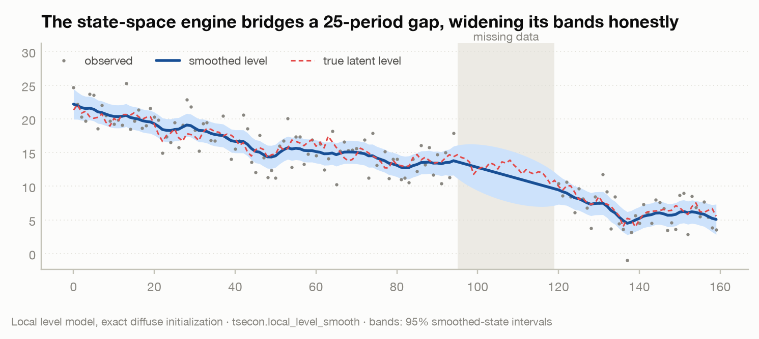
The figure shows exactly what the theory promises: the smoother bridges the gap with a sensible path, the 95% band balloons precisely where information is missing, and the true latent path — which the model never saw inside the gap — stays within the band. Estimating the two variances (rather than fixing them, as here) is one numerical optimization of the exact likelihood away, and that is what unobserved_components does — for the local level and for the whole of Harvey's structural family assembled from the same blocks:
fit = tsecon.unobserved_components(y)                     # local level, variances by exact-diffuse MLE
fit["params"], fit["se"]                                  # sigma2.irregular, sigma2.level
fit["level"], fit["level_var"]                            # smoothed level and its variance
bsm = tsecon.unobserved_components(y, level="lltrend", seasonal=12,
                                    cycle=True, damped_cycle=True, stochastic_cycle=True,
                                    exog=x, forecast_steps=12, forecast_exog=x_future)
bsm["at_boundary"]                                        # which variances piled up at zero
level names the trend block in statsmodels' vocabulary ("llevel", "lltrend", "strend", "rwdrift", "dtrend", ...), seasonal=s adds Harvey's dummy seasonal, freq_seasonal=[p] the trigonometric one, cycle=True the stochastic cycle, and every state starts exactly diffuse. On the Nile data the fitted variances reproduce the numbers Durbin and Koopman print (15099 and 1469.1); on the UK seat-belt data the basic structural model of Harvey and Durbin (1986) puts the slope and seasonal variances at zero — the pile-up of Shephard and Harvey (1990), reported as a flag with a NaN standard error rather than as a tiny estimate — and finds the law's effect as a regression coefficient with a standard error. The same machinery with the regression coefficients as random-walk states is tvp_regression(y, x): a time-varying-parameter regression whose zero-state-variance limit is recursive least squares, with the pile-up check on every coefficient variance. Fixed-parameter log-likelihoods, states, filtered variances, residuals and forecasts are pinned to statsmodels at 1e-8; the smoothed variances inside the diffuse period are pinned at the distance statsmodels' own two smoother implementations sit apart on the same model, because that — not 1e-8 — is what "as accurate as the reference" means where the reference disagrees with itself. The model card holds the grades.
⚠ Common mistake. Handling a missing observation by treating it as "observed with value 0" or by zero-weighting it. Both are wrong: the correct treatment is to skip the measurement update entirely and count only observed terms in the likelihood. A related implementation trap: initializing a nonstationary state (a random-walk level has no stationary distribution) with a "big number" variance approximation instead of the exact diffuse initialization — the likelihood constants come out wrong and cross-package comparisons silently break. tsecon uses exact diffuse initialization throughout.
When one line is not enough: regimes and thresholds
Everything so far assumes one set of dynamics governs the whole sample. Macroeconomic reality objects: recessions are not expansions run backward. US GDP falls fast and recovers slowly; unemployment rises in spikes and declines in long glides. Linear ARMA models — whose impulse responses are symmetric by construction — cannot represent this. Two families relax the assumption, distinguished by what triggers the switch.
Markov-switching AR (Hamilton, 1989) makes the trigger an unobserved discrete state \(s_t \in \{0, 1\}\) following a Markov chain:
Each regime has its own mean (and possibly variance and dynamics); the economy switches stochastically between them, and the model infers from the data alone the probability of being in each regime at each date. Hamilton's original application fit two regimes to postwar US GNP growth and found mean growth of roughly \(1.2\%\) per quarter in one regime and \(-0.4\%\) in the other, with both regimes persistent — and the smoothed probability of the low regime reproduced the NBER's recession dates almost exactly, without ever being shown them. That figure is one of the most famous in time series econometrics, and reproducing Hamilton's published estimates was the validation gate for tsecon.markov_switching_ar — a gate it now passes on Hamilton's own GNP series, means and transition probabilities and recession chronology together (replication).
Threshold AR (SETAR) (Tong and Lim, 1980) makes the trigger observable: the model switches when a lagged value of the series itself crosses a threshold \(\tau\):
("self-exciting" because the series triggers its own switches). STAR models (Teräsvirta, 1994) replace the hard switch with a smooth transition function, so the economy blends between regimes rather than jumping — natural for aggregates that sum many units crossing thresholds at different times, like real exchange rates under transaction costs.
When do you actually need these?
- Reach for Markov-switching when the regime is a latent classification you want the model to discover — business-cycle phases, high/low-volatility eras, policy regimes. The regime probabilities themselves are often the deliverable.
- Reach for SETAR/STAR when you can name the observable trigger — "dynamics change when the spread goes negative," "mean reversion kicks in when the real exchange rate deviates enough." The threshold estimate is interpretable in economic units.
- Stay linear when you have short samples or forecasting is the only goal. Nonlinear models need many visits to each regime to estimate it; with 150 quarterly observations and two recessions, the recession regime rests on a handful of data points, and the forecast gains over a good ARMA are often negligible.
All three ship: tsecon.markov_switching_ar for the latent-regime case, tsecon.setar with tsecon.setar_test for the hard threshold, and tsecon.star with tsecon.star_test for the smooth one — plus tsecon.star_eval, which scores a published \((\gamma, c)\) directly, because comparing SSRs across implementations is robust to optimizer differences and comparing parameters is not. Here is the workflow in the order the mistake box below insists on — test, then fit:
rng = np.random.default_rng(0)
n = 600
y = np.zeros(n)
e = rng.standard_normal(n)
for t in range(1, n):                    # SETAR(1): persistent below 0, transient above
    c, phi = (1.0, 0.6) if y[t-1] <= 0.0 else (-1.0, 0.2)
    y[t] = c + phi * y[t-1] + e[t]

lin = tsecon.setar_test(y, p=1, n_boot=499, seed=0)   # test BEFORE you fit
print(f"sup-F = {lin['stat']:.1f}   bootstrap p = {lin['p_value']:.3f}")

fit = tsecon.setar(y, p=1)
print(f"threshold = {fit['threshold']:.3f}  (delay {fit['delay']}, "
      f"{fit['n_low']}/{fit['n_high']} obs per regime)")
print("low  regime (c, phi):", np.round(fit["params_low"], 3))
print("high regime (c, phi):", np.round(fit["params_high"], 3))
sup-F = 204.8   bootstrap p = 0.002
threshold = 0.000  (delay 1, 336/263 obs per regime)
low  regime (c, phi): [0.877 0.488]
high regime (c, phi): [-0.965  0.119]
Read the threshold against the coefficients under it. The threshold lands on the truth to three decimals, because a threshold is superconsistent — it is pinned down faster than the coefficients on either side of it. Those coefficients, at \(T = 600\) with roughly 300 observations per regime, are recognizable but loose (0.49 against a true 0.6 below, 0.12 against 0.2 above): the "stay linear on short samples" bullet above, made concrete. And the p-value is a bootstrap p-value, not a \(\chi^2\) tail — the library refuses to compute the latter, for the reason the box below gives.
These families are estimation minefields — multimodal likelihoods requiring multistart optimization, unbounded likelihoods as a regime variance heads to zero, off-by-one traps in the regime smoother — which is why "reliability where statsmodels is fragile" is treated as the feature rather than the fine print. The visible form of that is honesty flags on every fit: star returns converged, se_valid, and gamma_at_boundary, which fires when the estimated transition speed runs to the top of its grid (numerically a hard threshold, and a signal to read \(\gamma\) as a lower bound) or pins at the bottom (numerically linear, with \(\gamma\) and the second regime's coefficients separately unidentified). A flat likelihood in \(\gamma\) is a real property of these models; the fit says so instead of printing a confident number.
⚠ Common mistake. Testing "linear vs. threshold" (or "one regime vs. two") with a standard likelihood-ratio test and \(\chi^2\) critical values. Under the null of linearity the threshold \(\tau\) (or the transition matrix) is unidentified — the Davies problem — and the LR statistic is not \(\chi^2\). Valid inference needs sup-type tests with simulated or bootstrapped critical values (Hansen, 1996). Every naive \(\chi^2\) p-value in this territory overstates the evidence for nonlinearity.
Long memory: when d refuses to be an integer
Return to the two rungs the ARIMA ladder actually offers for persistence. Either the series is stationary — \(d = 0\), and the autocorrelations decay geometrically, \(\rho_k \approx \phi^k\), so the memory of a shock is gone within a handful of lags — or it has a unit root — \(d = 1\), and a shock never fades at all. In the thermostat picture from the top of the chapter, that is a choice between a working thermostat and no thermostat. But some series behave as if the thermostat is real yet arbitrarily weak: it does pull the room back to the set point, so the series is mean-reverting, but it pulls ever more feebly, so a shock takes hundreds of periods to disappear. The autocorrelations of such a series decay hyperbolically — like \(k^{2d-1}\), a slow power law — not geometrically. Plot the ACF and it crawls toward zero across dozens of lags while never suggesting a unit root; run an ADF test and it rejects the unit root; fit an ARMA and it wants ever more AR terms, all with coefficients summing suspiciously close to one. The data are telling you the integer choice is too coarse.
Fractional integration (Granger and Joyeux, 1980; Hosking, 1981) fills the gap between the rungs by letting \(d\) be continuous. The device is to read integer differencing as a special case of a filter that makes sense for any real \(d\). The first-difference operator is \((1-L)\); differencing twice is \((1-L)^2 = 1 - 2L + L^2\); and the binomial theorem defines \((1-L)^d\) for fractional \(d\) through the same expansion carried to infinitely many terms,
For \(d = 1\) the weights are \(1, -1, 0, 0, \dots\) and you recover the ordinary first difference; for \(d = 2\) you recover \(1, -2, 1, 0, \dots\); but for \(d = 0.4\) the weights never terminate — they trail off slowly, and that slow tail is exactly the long memory. An ARFIMA(p, d, q) process (fractionally-integrated ARMA) applies this operator in place of the integer difference:
The memory parameter \(d\) now indexes a whole spectrum of persistence, not a binary switch. For \(0 < d < 0.5\) the process is stationary with autocorrelations decaying like \(k^{2d-1}\) — genuine long memory, summable nowhere yet finite in variance. At \(d = 0\) it collapses to plain ARMA (short memory); at \(d = 0.5\) the variance diverges and stationarity is lost; \(d < 0\) is antipersistence, the fingerprint of a series that has been over-differenced. The value \(d\) takes is an economically meaningful measurement, not a modeling nuisance — which is why it deserves to be estimated rather than assumed.
Where does this actually bite? The classic cases are exactly the series where practitioners kept noticing "near unit roots that reject the unit root":
- Realized volatility. Daily realized variance of equity returns is the textbook long-memory series, with \(d\) reliably near \(0.4\); the HAR model owes its success to approximating precisely this hyperbolic decay.
- Inflation. Inflation persistence sits in the awkward \(d \approx 0.3\)–\(0.5\) region — too persistent for a comfortable ARMA, not obviously \(I(1)\) — and the long-memory-versus-breaks debate over it is unresolved (see the frontier note below).
- Trading volume and bid-ask spreads. Market-microstructure series show the same slow ACF decay, a signature of the aggregation of many heterogeneous, slowly-adjusting traders.
Estimating \(d\) does not require committing to the full ARMA structure. The workhorses are semiparametric: they use only the low-frequency behavior of the periodogram, where the spectral density blows up like \(\lambda^{-2d}\) near the origin, and leave the short-run dynamics away from zero unmodeled. The GPH log-periodogram regression (Geweke and Porter-Hudak, 1983) regresses the log-periodogram at the lowest \(m\) Fourier frequencies on a simple transform of frequency; the slope is \(-d\) — a transparent OLS you can eyeball. The local Whittle estimator (Robinson, 1995) instead minimizes a concentrated Gaussian (Whittle) objective over the same low-frequency window; it is more efficient than GPH and is the modern default. Both share one tuning knob, the bandwidth \(m\): too large and the ARMA short-run structure leaks in and biases \(d\); too small and the estimate is noisy. The textbook default is \(m = \lfloor\sqrt{n}\rfloor\), and the standard discipline is to re-estimate across a grid of \(m\) and confirm \(d\) is stable.
Once you have \(d\), frac_diff earns its keep: apply \((1-L)^{\hat d}\) and the long memory is whitened out, leaving an approximately short-memory series that ordinary ARMA tools can finish off. That is the whole ARFIMA workflow — estimate \(d\) semiparametrically, fractionally difference, fit ARMA to the remainder — and it is the fractional analogue of "difference, then fit ARMA" that defines ARIMA. The contrast with the ARIMA section is the entire point: ARIMA forces \(d\) to be an integer you pick with a unit-root test; fractional integration lets the data choose a non-integer \(d\) you estimate.
Here is the full loop — simulate an ARFIMA(0, d, 0) by fractionally integrating white noise, recover \(d\) two ways, and watch the ACF collapse from hyperbolic decay to nothing under fractional differencing:
import numpy as np
import tsecon

rng = np.random.default_rng(20)
n, d_true = 6000, 0.40
eps = rng.standard_normal(n)
x = tsecon.frac_integrate(eps, d_true)          # ARFIMA(0, d, 0): known long memory

# estimate d two ways, at the textbook bandwidth m = floor(sqrt(n))
gph = tsecon.long_memory_d(x, method="gph")             # Geweke-Porter-Hudak (1983)
lw  = tsecon.long_memory_d(x, method="local_whittle")   # Robinson (1995)
print(f"true d          = {d_true}")
print(f"GPH d           = {gph['d']:.3f}  se {gph['se']:.3f}  (m={gph['m']})")
print(f"local-Whittle d = {lw['d']:.3f}  se {lw['se']:.3f}  (m={lw['m']})")

# whiten with the local-Whittle estimate, then compare the ACF before/after
white = tsecon.frac_diff(x, lw["d"])
acf_x     = tsecon.acf(x,     nlags=20)["acf"]
acf_white = tsecon.acf(white, nlags=20)["acf"]
print("\nlag :   memory   whitened")
for k in (1, 5, 10, 20):
    print(f"{k:>3} :   {acf_x[k]:+.3f}   {acf_white[k]:+.3f}")

# does any structure survive the whitening?
print("\nLjung-Box(20) p, memory series :",
      f"{tsecon.ljung_box(x,     nlags=20)['lb_pvalue'][-1]:.3g}")
print("Ljung-Box(20) p, whitened      :",
      f"{tsecon.ljung_box(white, nlags=20)['lb_pvalue'][-1]:.3g}")
true d          = 0.4
GPH d           = 0.435  se 0.080  (m=77)
local-Whittle d = 0.451  se 0.063  (m=77)

lag :   memory   whitened
  1 :   +0.606   -0.041
  5 :   +0.375   -0.021
 10 :   +0.317   +0.002
 20 :   +0.255   +0.009

Ljung-Box(20) p, memory series : 0
Ljung-Box(20) p, whitened      : 0.0455
Read the ACF column top to bottom: the memory series is still correlated at \(+0.26\) twenty lags out — a decay no stationary ARMA would produce with a lag-1 of only \(0.61\) — while the fractionally-differenced series sits within sampling noise of zero everywhere. The two estimators land at \(0.44\) and \(0.45\), both within about one standard error of the true \(0.40\) (semiparametric estimators buy their freedom from the ARMA structure with wide bands — note the \(se\) of \(0.06\)–\(0.08\) even at \(n = 6000\)). And because local Whittle landed slightly high, frac_diff differenced a touch too hard: the whitened series shows a small negative lag-1 autocorrelation (\(-0.041\)), the mild-over-differencing tell, which is exactly why the Ljung-Box p on the whitened series is borderline rather than comfortably large. That residual is short-range and tiny — precisely the mopping-up job an ARMA(p, q) on the whitened series is for. See the long-memory model card for the estimator conventions, the exact se formulas, and frac_integrate as the exact inverse of frac_diff.
⚠ Common mistake. Choosing the bandwidth \(m\) too large "to use more data." Semiparametric \(d\) estimation is local to the origin on purpose; as \(m\) grows, the ARMA short-run dynamics at higher frequencies contaminate the regression and bias \(\hat d\) — usually upward, manufacturing long memory that is really just AR persistence. Report \(\hat d\) across a grid of \(m\), not a single value. And do not read an estimate near \(0.5\) as a verdict on stationarity: the band almost always straddles the boundary, and neither GPH nor local Whittle is built to test \(d = 1\) — that is a unit-root test's job.
The frontier
Long memory beyond the stationary window. The previous section covers the stationary case (\(0 < d < 0.5\)) and its shipped estimators; the research edge lies just outside it. Estimating \(d\) when the series is nonstationary (\(d \ge 0.5\)) breaks GPH and ordinary local Whittle, and needs the exact local Whittle estimator (Shimotsu and Phillips, 2005), valid across the stationary boundary. Full ARFIMA(p, d, q) maximum likelihood via Sowell's (1992) exact autocovariances jointly estimates \(d\) with the ARMA parameters but is numerically delicate as \(d \to 0.5\). And the genuinely open problem is identification: long memory and structural breaks are nearly observationally equivalent (Diebold and Inoue, 2001) — a short-memory process with occasional mean shifts reproduces every classic long-memory signature, hyperbolic ACF decay included — so a significant \(\hat d\) is never on its own proof of long memory rather than a wandering mean, and distinguishing the two on realistic sample sizes remains unsolved in general.
Elsewhere on the research edge. Score-driven (GAS/DCS) models (Creal, Koopman and Lucas, 2013) make parameters time-varying through the score of the likelihood, giving robust filters that automatically discount outliers — the corner of this list that has since crossed into the library, as dcs_local_level (a robust cousin of this chapter's local level, listed below) and gas_volatility (score-driven volatility, chapter 6). Bayesian TVP models with global-local shrinkage priors (Bitto and Frühwirth-Schnatter, 2019) let the data decide which coefficients drift — the current standard in empirical macro. Testing for the number of Markov regimes is finally practical via Carrasco, Hu and Ploberger (2014). Mixed causal-noncausal AR models (Lanne and Saikkonen, 2011; Gouriéroux and Zakoïan, 2017) use roots inside the unit circle, identified through non-Gaussianity, to capture bubble episodes that explode and collapse. And an ecosystem-wide embarrassment remains open: default prediction intervals nearly everywhere ignore parameter and selection uncertainty and are systematically too narrow — dramatically so near unit roots and for \(T < 100\); bootstrap and conformal methods are the frontier fixes, and the distribution-free half of that repair ships here as conformal_forecast/conformal_backtest (split, EnbPI, and adaptive conformal inference).
The Module 02 roadmap covers this terrain in tiers, and the first two of them have largely landed: the ARMA/SARIMA stack and auto-ARIMA from the core tier, and SETAR/STAR, Markov-switching, Bai-Perron breaks, the GPH and local-Whittle long-memory entry points, and the score-driven filters from the standard and advanced ones, all ship today. What the tiers still hold is what the roadmap list below names — regARIMA, fitted unobserved components, Sowell ARFIMA and the exact local Whittle, shrinkage TVP — each gated on reproducing published numbers (Hamilton's GNP estimates, the airline model, the Nile variances) rather than matching another package's defaults, which is the bar the shipped half was held to.
Which method when
| Situation | Reach for | Because |
|---|---|---|
| Short-horizon forecast of a stationary series, no covariates | AR(p), order by AICc | Cheapest credible momentum model; hard to beat at h = 1–4 |
| ACF cuts off sharply; shocks visibly transient | MA(q) or ARMA(1,1) | Finite shock memory is what MA terms are for |
| Trending level series (GDP, prices) | ARIMA with d chosen by check_stationarity |
Difference first; unit-root tests, not AIC, pick d |
| Monthly/quarterly data with stable seasonality | SARIMA — start at the airline model (0,1,1)(0,1,1)ₛ | Four parameters cover a remarkable share of seasonal economic series |
| Many series to forecast automatically | auto_arima or auto_ets, then residual checks |
Disciplined search beats hand-tuning at scale — but never skip diagnostics |
| Trend + seasonal forecasting, fast and robust | Theta (theta_forecast) or the ETS taxonomy (ets_fit, auto_ets) |
M3-competition-grade accuracy at trivial cost |
| Noisy measurements of an underlying level; gaps in the data | Local level/trend via unobserved_components (local_level_smooth at fixed variances) |
Kalman filter handles missing data exactly, with honest uncertainty; the variances are estimated, and a variance that piles up at zero is flagged |
| Trend + seasonal + cycle decomposition, an intervention effect, or a regression whose coefficients drift | unobserved_components(level=..., seasonal=..., cycle=..., exog=...), tvp_regression |
Harvey's structural models and the TVP regression on one exact-diffuse Kalman engine, validated against statsmodels |
| Small sample, persistence near a unit root | Exact MLE, never CSS or Yule-Walker | Initial conditions carry real information; moment methods bias toward stationarity |
| Asymmetric dynamics with a latent phase (recessions) | markov_switching_ar |
Infers regime probabilities from the data; the probabilities are the deliverable |
| Dynamics change at a nameable observable trigger | setar (hard switch) or star (smooth), after setar_test/star_test |
Interpretable threshold in economic units; test linearity properly first |
| The mean shifts at unknown dates rather than switching back and forth | bai_perron |
Breaks are one-way regime changes; estimating their dates beats dummying by eye |
| Autocorrelations decay too slowly for ARMA but the series reverts | long_memory_d, then frac_diff |
Fractional d is the honest middle ground between I(0) and I(1) — but rule out breaks |
| A few contaminated observations are dragging the level around | dcs_local_level |
A bounded score discounts outliers where the Kalman gain would chase them |
What tsecon implements today
Available now in Python (import tsecon):
ar_loglik(y, coeffs, sigma2, intercept=0.0)— exact Gaussian AR(p) log-likelihood via the state-space form with stationary initialization; the exact-MLE kernel this chapter's estimation section is built onlocal_level_smooth(y, sigma2_eps, sigma2_eta)— exact-diffuse Kalman filter and smoother for the local level model; NaNs handled natively as missing dataunobserved_components(y, level="llevel", seasonal=None, freq_seasonal=None, cycle=False, exog=None, forecast_steps=0, ..., autoregressive=None, cycle_init=None, mle_regression=None)— Harvey's structural models by exact-diffuse MLE: every statsmodels level/trend specification, dummy and trigonometric seasonals, the (damped) stochastic cycle, an AR(p) component (autoregressive=p), regressors as parameters or —mle_regression=False— as diffuse states with GLS coefficient paths, the stationary (Lyapunov) initialization of a damped cycle (cycle_init="stationary", which removes the cycle's low-frequency likelihood singularity), missing data, smoothed and filtered components with variances, forecasts with variances, and the pile-up flag on every variance. The last two switches change the definition of the log-likelihood, so it is not comparable across themtvp_regression(y, x, constant=True)— regression with random-walk coefficients on the same Kalman machinery: filtered and smoothed coefficient paths with variances, the observation and state variances by MLE, and the pile-up check (its zero-variance limit is recursive least squares)arima_fit(y, p, d, q, seasonal=None, constant=True, forecast_steps=0, conf_alpha=None)— exact-MLE ARIMA(p,d,q) and, throughseasonal=(P, D, Q, s), SARIMA: params, log-likelihood, AIC/BIC, residuals, and multi-step forecasts with correctly integrated-back intervals. Note the default: a constant is fitted, which for \(d \ge 1\) is a drift — passconstant=Falsewhen you do not want oneauto_arima(y, seasonal_period=0, ic="aicc", stepwise=True, ...)— the Hyndman-Khandakar (2008) search on that same exact-MLE engine, in the order this chapter insists on:Dby the seasonal-strength rule,dby successive KPSS tests, then a stepwise (or exhaustive) walk over \((p, q, P, Q)\) at fixed differencingmarkov_switching_ar(y, k_regimes=2, order=1, switching_variance=True)— Hamilton (1989) MS-AR by EM: the transition matrix, per-regime means and variances, expected durations, and the full filtered (Hamilton) and smoothed (Kim 1994) regime-probability paths.filtered_probis the real-time object;smoothed_probconditions on the whole sample, so it dates recessions in hindsight and must not be read as a live callsetar(y, p, delay=1, trim=0.15)andsetar_test(y, p, delay=1, trim=0.15, n_boot=499)— two-regime SETAR by concentrated least squares (Tong-Lim 1980; Hansen 1997), and the Hansen (1996) sup-F linearity test p-valued by the fixed-regressor wild bootstrap, because the Davies problem flagged in the regimes section above makes a naive \(\chi^2\) p-value wrongstar(y, p, model="lstar"|"estar", delay=1),star_eval(y, p, gamma, c, ...),star_test(y, p, delay=1)— smooth-transition AR by concentrated NLS over a standardized-γ grid, the fixed-\((\gamma, c)\) scorer, and the Teräsvirta (1994) modeling cycle: the LM3 linearity test plus the H03/H02/H01 sequence that picks LSTAR against ESTARbai_perron(y, x, max_breaks=5, trim=0.15)— multiple structural breaks: the global partitions by dynamic programming, the number of breaks by sequential supF(ℓ+1|ℓ), per-regime OLS, and Bai (1997) break-date confidence intervals (withsup_f_testfor the single-break screen)long_memory_d(x, m=None, method="gph"|"local_whittle")— the two semiparametric estimators of \(d\) from the long-memory section, withfrac_diff/frac_integratefor fractional differencing and its exact inverse; this is the code that section runsdcs_local_level(y, density="t"|"laplace"|"gaussian")— the score-driven robust local level (Harvey 2013; Harvey-Luati 2014): an outlier-resistant cousin of the Kalman local level above, with the Gaussian case exactly the steady-state Kalman filter, so the nested control is checkable- Identification and diagnostics used throughout the chapter:
acf,pacf,ljung_box,jarque_bera,arch_lm - Differencing decisions:
adf,kpss,check_stationarity, plus the order advisorsndiffs(the KPSS sequence auto-ARIMA uses for \(d\)) andnsdiffs(seasonal strength for \(D\)) - The exponential-smoothing family:
ets_fit(all 30 ETS models, exact or simulated prediction intervals) andauto_ets(the AICc candidate search), plus its benchmarktheta_forecast, withaccuracyanddm_testfor honest evaluation
Built in Rust (tsecon-arima crate), all of it bound:
- The ARIMA(p,d,q) engine — seasonal
(P, D, Q, s)orders included — ships in Python asarima_fitabove (exact MLE, log-likelihood, residuals, integrated-back forecast intervals), and since 0.11 so does the CSS estimator, asarima_fit(..., method="css")— its conditional log-likelihood, conditional-Hessian standard errors and conventions are on the ARIMA card
Roadmap (docs/roadmap/02-univariate.md):
- Regression with ARMA errors (regARIMA); Hannan-Rissanen starts and the Monahan reparameterization as public API
- ARFIMA (Sowell exact MLE); the exact local Whittle estimator (Shimotsu-Phillips 2005), which stays valid across the \(d \ge 0.5\) boundary where GPH and ordinary local Whittle break
- Hansen (1997, 2000) confidence sets for the SETAR threshold, and a test for the number of Markov regimes (Carrasco-Hu-Ploberger 2014) — the two inference gaps left open by the regime models that now ship above
Further reading
- Box, G. E. P. and G. M. Jenkins (1970), Time Series Analysis: Forecasting and Control, Holden-Day. The book that created the ARIMA methodology, the airline model, and the identify-estimate-check loop this chapter walks.
- Wold, H. (1938), A Study in the Analysis of Stationary Time Series, Almqvist & Wiksell. The decomposition theorem that explains why ARMA models can approximate any stationary process — the license for the whole family.
- Kalman, R. E. (1960), "A New Approach to Linear Filtering and Prediction Problems," Journal of Basic Engineering. The filter, from outside economics entirely; sixty-five years later it is the estimation engine of this whole module.
- Hamilton, J. D. (1989), "A New Approach to the Economic Analysis of Nonstationary Time Series and the Business Cycle," Econometrica. Markov-switching AR and the recession-probability plot that launched a literature.
- Tong, H. and K. S. Lim (1980), "Threshold Autoregression, Limit Cycles and Cyclical Data," Journal of the Royal Statistical Society B. The founding SETAR paper; nonlinear time series as a practical toolkit begins here.
- Teräsvirta, T. (1994), "Specification, Estimation, and Evaluation of Smooth Transition Autoregressive Models," Journal of the American Statistical Association. The complete STAR modeling cycle — test, select, estimate — still the standard workflow.
- Granger, C. W. J. and R. Joyeux (1980), "An Introduction to Long-Memory Time Series Models and Fractional Differencing," Journal of Time Series Analysis. Fractional integration's founding paper (with Hosking, 1981, Biometrika, its independent twin).
- Hyndman, R. J., A. B. Koehler, R. D. Snyder and S. Grose (2002), "A State Space Framework for Automatic Forecasting Using Exponential Smoothing Methods," International Journal of Forecasting. The paper that turned exponential smoothing from methods into models.
- Hyndman, R. J. and Y. Khandakar (2008), "Automatic Time Series Forecasting: The forecast Package for R," Journal of Statistical Software. The auto-ARIMA and AutoETS algorithms every automatic-forecasting system now descends from.
- Durbin, J. and S. J. Koopman (2012), Time Series Analysis by State Space Methods, 2nd ed., Oxford University Press. The definitive state-space text: exact diffuse initialization, smoothing, missing data — the conventions tsecon implements.