Chapter 8 — Structural Identification: From Correlation to Cause
Part of The tsecon Guide to Time Series Econometrics. Chapters mirror the library's modules; code runs against the current Python API unless marked otherwise.
Prerequisites: Chapter on VARs (fitting, impulse responses, forecast-error variance decompositions) and comfort with OLS and covariance matrices.
You will learn:
- Why the shocks a VAR estimates are correlated mixtures of the shocks economists care about, and why no amount of data fixes that on its own
- What "identification" means precisely: the rotation problem, and how many assumptions you owe before an impulse response is causal
- The major identification schemes — recursive, long-run, sign, heteroskedasticity, narrative, and instrument-based — each with its maintained assumptions and its classic failure mode
- How the modern instrument-based approaches connect VARs to local projections, and why the two estimate the same thing
- How to choose a scheme for your question, and what honest inference looks like when identification is a set rather than a point
The idea
Here is the question that launched forty years of macroeconometrics: what does a monetary tightening do to output? The Federal Reserve raises its policy rate; a year later, unemployment is higher. Did the rate hike cause that? Or did the Fed raise rates because it saw inflation and an overheating economy coming — in which case the correlation between rates and future output tells you about the Fed's reaction, not about the Fed's power?
This is the simultaneity problem, and in macro data it is everywhere. The policy rate responds to the economy within the quarter; the economy responds to the policy rate within the quarter. Demand shifts move prices and quantities; so do supply shifts. When you fit a VAR — the workhorse multivariate model from the previous chapters — you get residuals, one per equation per period. It is tempting to call the residual in the interest-rate equation "the monetary policy shock." It is not. It is the part of the rate that the VAR's lags could not predict — a mixture of the Fed's genuine surprise decisions and the Fed's same-quarter reaction to demand surprises, supply surprises, financial surprises, and everything else that hit the economy that quarter. The residuals across equations are correlated with each other precisely because they share these underlying causes.
Think of it like listening to a recording of an orchestra made with one microphone per seat. Every microphone picks up every instrument — the violin mic mostly violin, but also the timpani two rows back. The VAR residuals are the microphone tracks: correlated blends. The structural shocks — the pure monetary shock, the pure demand shock — are the individual instruments. Identification is the problem of unmixing the tracks. And here is the uncomfortable truth this chapter is built around: the data alone cannot do the unmixing. The recording is consistent with many different seatings of the orchestra. You must bring outside information — economic theory, institutional knowledge, historical documents, or extra data such as a measured instrument — to pin down which unmixing is the true one. Every identification scheme in this chapter is a different kind of outside information, and each one buys you causality at the price of an assumption you must be prepared to defend.
This chapter is the guide's tour of that territory — and it maps directly onto the library module that tsecon considers its headline differentiator, because no maintained Python package covers modern SVAR identification today. The check is concrete: statsmodels 0.15 ships SVAR, which does short-run A/B parameter restrictions and nothing else — no sign restrictions, no zero-plus-sign sampler, no proxy/external-instrument scheme, no narrative or robust-Bayes layer.
Reduced form versus structure: the rotation problem
A practitioner cares about this section because it is the accounting identity of the whole subject: it tells you exactly how many assumptions you owe, and why "let the data decide" is not an available option.
Write the reduced-form VAR from the multivariate chapter as
where \(y_t\) is an \(n \times 1\) vector of observables (say output growth, inflation, and a policy rate), the \(A_j\) are estimated lag-coefficient matrices, and \(u_t\) is the vector of one-step-ahead forecast errors — the reduced-form innovations. Everything here is estimable by OLS and, given enough data, known.
The structural VAR (SVAR) asserts that these innovations are linear combinations of underlying economic shocks:
where \(\varepsilon_t\) collects the structural shocks — mutually uncorrelated, unit variance by normalization — and the \(n \times n\) impact matrix \(B\) says how much each structural shock moves each variable within the period. Column \(j\) of \(B\) is the impact response of the whole system to shock \(j\); combined with the estimated lag dynamics it generates the structural impulse response functions (IRFs) that answer causal questions.
Now count. The data reveal \(\Sigma_u = BB'\). A symmetric \(n \times n\) covariance matrix contains \(n(n+1)/2\) distinct numbers. The matrix \(B\) contains \(n^2\) unknowns. The shortfall is
numbers that the data cannot deliver. For a 3-variable VAR that is 3 missing restrictions; for a 7-variable monetary system, 21.
The geometric version of the same fact is the rotation problem. Suppose \(B\) satisfies \(BB' = \Sigma_u\). Take any orthogonal matrix \(Q\) (a rotation: \(QQ' = I\)). Then \(\tilde{B} = BQ\) satisfies
equally well. Every rotation of a valid impact matrix is another valid impact matrix, producing identical reduced-form fit, identical forecasts, identical likelihood — and different causal stories. The set of \(n \times n\) orthogonal matrices has dimension exactly \(n(n-1)/2\): the rotation problem is the counting shortfall, seen geometrically. (For \(n = 2\) that dimension is 1 — every rotation is a single angle \(\theta\) — which is why bivariate examples are the standard way to see an identified set: as \(\theta\) sweeps the circle, the implied impact matrices trace out every observationally equivalent model.) Two researchers with the same data and the same VAR can report opposite signs for the effect of money on output, and no statistical test can adjudicate between them, because their models are observationally equivalent.
The equivalence is easy to watch happen. Fit a VAR, take any admissible impact matrix, rotate it by any angle you like, and confirm that the implied residual covariance has not moved:
import numpy as np
import tsecon

rng = np.random.default_rng(0)
mix = np.array([[1.0, 0.0, 0.0], [0.5, 1.0, 0.0], [0.3, 0.4, 1.0]])
y = rng.standard_normal((300, 3)) @ mix.T        # three correlated series

r = tsecon.var_fit(y, lags=1)
Sigma = np.array(r["sigma_u"])
B = np.linalg.cholesky(Sigma)                    # one admissible impact matrix

theta = 0.7                                      # any angle at all
Q = np.array([[ np.cos(theta), np.sin(theta), 0.0],
              [-np.sin(theta), np.cos(theta), 0.0],
              [ 0.0,           0.0,           1.0]])
B_tilde = B @ Q                                  # a different causal story...
print(np.abs(B_tilde @ B_tilde.T - Sigma).max()) # ...identical fit: ~1e-16
B and B_tilde imply different shocks, different impulse responses, different history — and the data cannot tell them apart.
Identification therefore means: impose at least \(n(n-1)/2\) credible restrictions that select the true \(B\) (point identification), or impose weaker restrictions that shrink the set of admissible \(B\)'s and be honest that you end with a set (set identification). Everything that follows is a catalog of where those restrictions can legitimately come from.
⚠ Common mistake: treating the reduced-form innovations \(u_t\) themselves as shocks — "the residual in the interest-rate equation is the policy shock." Unless \(B\) happens to be diagonal (it never is; the residuals are correlated), each \(u_{it}\) is a blend of all \(n\) structural shocks, and IRFs computed from unorthogonalized innovations answer no causal question at all.
Recursive identification: what an ordering buys you
The oldest and still the most common answer, from Sims (1980): assume the impact matrix is lower triangular. Economically, you assert a causal ordering within the period: the first variable responds to no other shock on impact, the second responds contemporaneously only to the first, and so on. The last variable — often the policy rate — responds to everything on impact, but nothing responds to it until next period.
This is attractive because it is exactly enough: a lower-triangular \(B\) has \(n(n+1)/2\) free elements, matching what \(\Sigma_u\) delivers, and there is a unique lower-triangular matrix with positive diagonal satisfying \(BB' = \Sigma_u\) — the Cholesky factor:
No optimization, no sampling; one matrix decomposition and you have point-identified shocks. In the classic monetary VAR of Christiano, Eichenbaum, and Evans (1999), slow-moving variables (output, prices) are ordered before the federal funds rate: the identifying claim is that production and pricing decisions cannot react to a policy surprise within the same quarter — plausible if firms set production plans and prices in advance — while the Fed can react to output and prices within the quarter, which is exactly what its information set allows. When the timing claim is institutionally grounded like this, Cholesky is defensible. When the ordering is chosen by habit, it is an unexamined assumption wearing a lab coat.
tsecon's var_irf computes orthogonalized (Cholesky) IRFs today. Here is the whole loop on synthetic data with a known recursive structure, so you can watch identification succeed when its assumption is true:
import numpy as np
import tsecon

rng = np.random.default_rng(42)
T, n = 400, 3
eps = rng.standard_normal((T, n))     # structural shocks: demand, output, policy

B0 = np.array([[1.0, 0.0, 0.0],       # demand reacts to nothing on impact
               [0.5, 1.0, 0.0],       # output absorbs demand within the period
               [0.3, 0.4, 1.0]])      # the policy rate leans against both
A1 = np.array([[0.5, 0.0, -0.2],
               [0.1, 0.4,  0.0],
               [0.0, 0.1,  0.5]])

y = np.zeros((T, n))
for t in range(1, T):
    y[t] = A1 @ y[t - 1] + B0 @ eps[t]

irf = tsecon.var_irf(y, lags=1, horizon=16)   # irf[h][i][j]: response of i to shock j
print(np.round(np.array(irf[0]), 2))          # impact matrix -> recovers B0
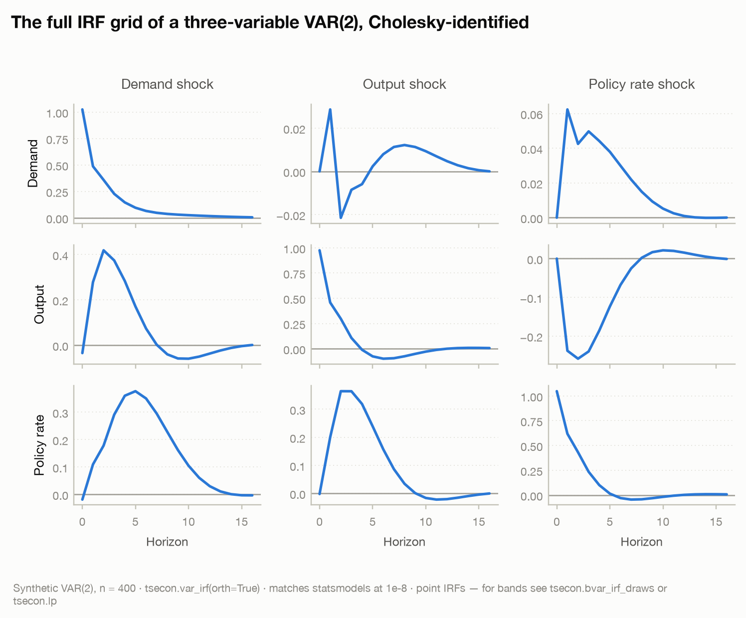
Because the true impact matrix is lower triangular and the ordering in the data matches it, the estimated impact step irf[0] reproduces B0 (the Cholesky factor is unique). The gallery's VAR section runs exactly this kind of system — demand moves first, output responds with a lag, the policy rate leans against both — and the estimated IRF grid recovers the built-in story:
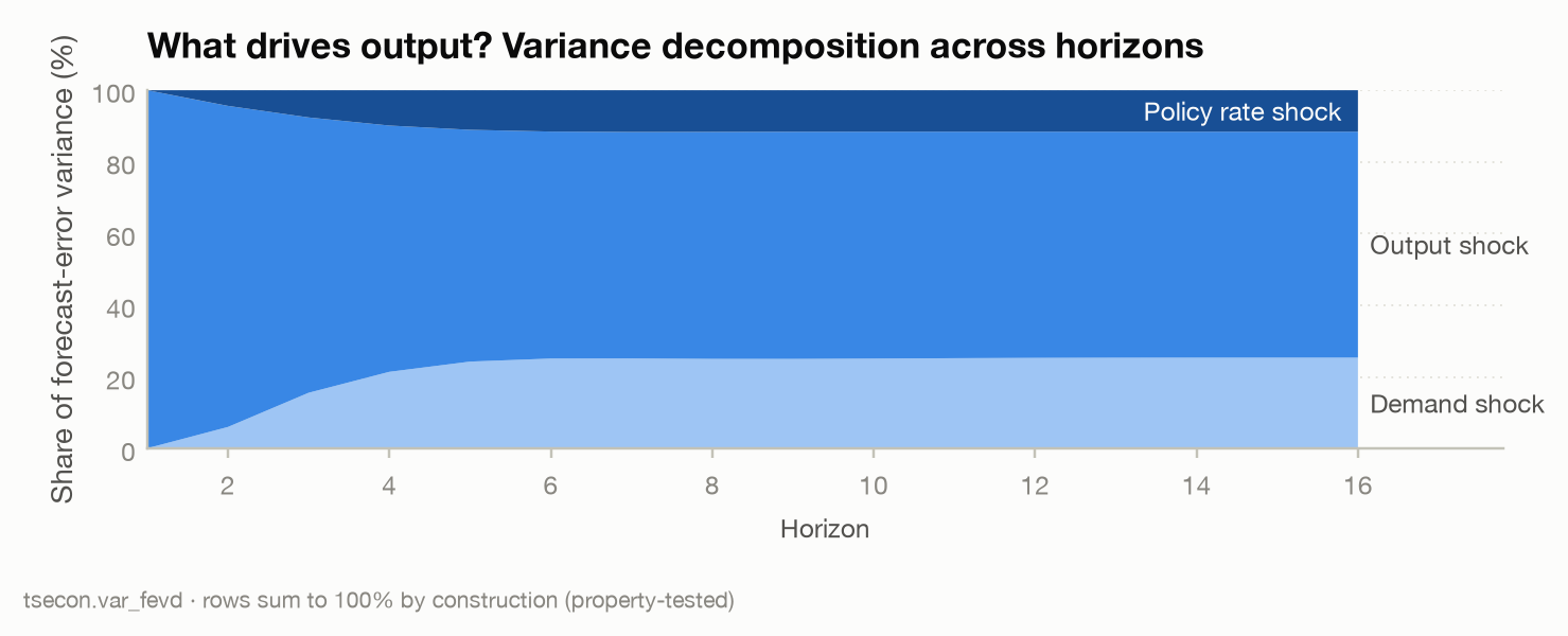
The companion decomposition question — what share of each variable's forecast errors does each shock explain? — is the forecast-error variance decomposition, also identified by the same Cholesky factor:
fevd = np.array(tsecon.var_fevd(y, lags=1, horizon=16))  # [horizon][variable][shock]
print(np.round(fevd[8], 2))         # shares at horizon 8; each row sums to 1
Now the honesty check: the ordering is the identification. Permute the variables and you get a different causal story from the same data:
perm = [2, 1, 0]                                    # policy ordered first
y_perm = np.ascontiguousarray(y[:, perm])
irf_perm = tsecon.var_irf(y_perm, lags=1, horizon=16)
print(np.round(np.array(irf_perm[0]), 2))           # a different impact matrix
Both runs fit the data identically. Only the first matches how the data were generated — and with real data, nothing inside the sample tells you which ordering that is. The module spec plans cheap ordering sweeps precisely so this sensitivity is a one-liner rather than an afterthought.
⚠ Common mistake: "I tried all orderings and the IRF barely changed, so identification doesn't matter here." Ordering-insensitivity only means the residual correlations are small; it is evidence about \(\Sigma_u\), not about causality. Conversely, "robustness across orderings" cannot rescue a system where no recursive ordering is economically defensible — with financial variables like stock returns or spreads in the VAR, every slow-fast ordering is wrong, because asset prices react to everything within the day and the macro variables plausibly react to them. That is exactly the case that pushes you toward heteroskedasticity or external instruments below.
Long-run restrictions: the Blanchard-Quah decomposition
Sometimes theory is silent about timing within a quarter but loud about the long run. The canonical example is Blanchard and Quah (1989): virtually any macro model implies that demand shocks have no permanent effect on the level of output — in the long run, output is pinned down by technology and supply — while supply shocks do have permanent effects. That is a restriction you can impose without taking any stand on who moves first within the quarter.
Formally, let \(A(L) = I - A_1 L - \cdots - A_p L^p\), so \(A(1) = I - A_1 - \cdots - A_p\). The cumulative (long-run) effect of the structural shocks on the levels of the variables is
Blanchard-Quah imposes that \(\Theta(1)\) is lower triangular — in the bivariate (output growth, unemployment) system: the second ("demand") shock has zero long-run effect on output. That again supplies exactly \(n(n-1)/2\) restrictions, and the solution is closed-form:
It is a Cholesky decomposition applied at the infinite horizon instead of at impact — an elegant trick, and the origin of the whole supply/demand decomposition literature.
The scheme's weakness is equally famous. \(A(1)^{-1}\) blows up as the VAR's largest roots approach one — precisely the region macro data live in — so small estimation errors in the lag coefficients become enormous errors in the long-run matrix. Faust and Leeper (1997) showed that in finite samples the long-run restriction can have essentially no bite: sizable short-run misidentification is consistent with the long-run constraint holding. The practical readings: check the estimated VAR's characteristic roots before trusting a long-run scheme (in the statsmodels convention var_fit follows, stability requires every root to lie outside the unit circle — a root modulus close to 1 is the warning sign), prefer the vector-error-correction formulation when cointegration is plausible, and treat Blanchard-Quah conclusions as fragile whenever persistence is high. tsecon's implementation (Module 06) will warn on near-unit roots by default, because the failure is silent otherwise. Until then, long_run_svar_bands reports the full-sample min_root and counts the explosive bootstrap refits in n_unstable_draws.
tsecon ships the Blanchard-Quah decomposition today as long_run_svar — closed-form, the analog of R's vars::BQ. Here it is on a synthetic bivariate system (output growth, unemployment) built so a "supply" shock has a permanent effect on the level of output and a "demand" shock does not:
import numpy as np
import tsecon

rng = np.random.default_rng(0)
T = 400
es = rng.standard_normal(T)     # supply (permanent)
ed = rng.standard_normal(T)     # demand (transitory)
dy = np.zeros(T); u = np.zeros(T)
for t in range(2, T):
    dy[t] = 0.2 * dy[t - 1] + es[t] + 0.5 * ed[t] - 0.5 * ed[t - 1]
    u[t] = 0.6 * u[t - 1] - 0.3 * es[t] + 0.7 * ed[t]
bq_data = np.column_stack([dy, u])

bq = tsecon.long_run_svar(bq_data, lags=4, horizon=20)
print("long-run matrix (lower-triangular by construction):")
print(np.round(np.asarray(bq["long_run"]), 4))
cum = np.asarray(bq["cumulative_irf"])      # [h][response][shock]
print("output's cumulative response to the demand shock, h = 0, 4, 20:",
      np.round(cum[[0, 4, 20], 0, 1], 6))
long-run matrix (lower-triangular by construction):
[[ 1.2008  0.    ]
 [-0.3017  1.6799]]
output's cumulative response to the demand shock, h = 0, 4, 20: [ 3.75038e-01 -1.11681e-01 -1.10000e-05]
The imposed zero sits in the upper-right of the long-run matrix, and output's cumulated response to the demand shock returns to zero by horizon 20 — the neutrality, echoed back as a built-in sanity check. Pass a custom restrictions=[(variable, shock), …] list for a non-recursive long-run pattern (normalize flips the sign convention, and impact_signs=[(variable, shock), …] anchors a shock's sign on its impact response; Blanchard-Quah's expansionary demand shock is impact_signs=[(0, 1)]). The fluent tsecon.svar(...).identify_long_run(...) wrapper with an automatic near-unit-root warning remains a Module 06 roadmap item.
⚠ Common mistake: forgetting that with differenced variables in the VAR, the interesting IRF is the cumulated one (the response of the level), and cumulating after orthogonalization is not the same as orthogonalizing cumulated responses if done carelessly.
long_run_svarreturnscumulative_irfalongsideirfso the level response of output to a demand shock visibly returns to zero — the restriction you imposed — without you re-deriving it.
On real data. The Blanchard-Quah replication runs long_run_svar with the paper's own design — US output growth demeaned around the 1974Q1 productivity break, detrended unemployment, eight lags — on the bundled 1959–2009 macrodata (a design replication at figure resolution: the paper's 1948–1987 GNP vintage is unreachable, so it pins shapes, not digits) and recovers the published shapes: a demand disturbance's effect on output peaks after three quarters (+1.10) and is gone by ten years (−0.004 at h = 40), the supply effect settles at a permanent +0.48, unemployment mirrors output, and demand accounts for about 90% of output's forecast-error variance a year out. The page also shows what the scheme hinges on: drop the break in mean growth and the long-run restriction reads the post-1973 slowdown as one enormous supply disturbance, collapsing demand's share of output variance from 97% to about 40% — the Faust-Leeper fragility above, made concrete. Its bands come from long_run_svar_bands, a residual bootstrap that re-identifies inside every draw, with Kilian's bias correction and a delta-method arm beside it. Its historical decomposition is historical_decomposition(identification="impact", impact=long_run_svar(...)["impact"]). The model card's per-cell coverage table is worth reading before you quote a band. On the page's own VAR(8) taken as truth, no arm covers every cell: the plain bootstrap band on output's hump-shaped response to demand covers 0.56–0.68 at h ≤ 8 against a nominal 0.90, and only the delta arm stays above 0.81 there.
Sign restrictions: honest bands, not points
Recursive and long-run schemes deliver a point — one \(B\) — by imposing hard zeros that many economists find too strong. Uhlig (2005) proposed a humbler kind of outside information: signs. A contractionary monetary policy shock, whatever else it does, should raise the federal funds rate, lower prices, and lower nonborrowed reserves for a few quarters. Notice what is deliberately left out: the response of output is unrestricted, because that is the question. Any rotation whose IRFs violate the signs is rejected; every rotation that satisfies them is kept.
The algorithm is direct. Given the reduced form, the admissible impact matrices are
Draw random rotations \(Q\) uniformly (from the Haar distribution — the uniform distribution on the orthogonal group), keep the ones whose IRFs pass, and summarize the survivors. Because signs are inequalities, not equalities, they do not pin down a point: you end with a set of models, not one. This is called set identification, and it changes what honest reporting means. The output is a band of IRFs that are all fully consistent with both the data and your assumptions — the width of that band is a finding. If the output response to a sign-identified monetary shock spans zero, that is the paper's result, not a nuisance to be narrowed by prettier plotting. (Uhlig's own punchline was exactly this: under agnostic sign restrictions, the contractionary effect of money on output is far less certain than the Cholesky consensus suggested.)
Two honesty rules come with the method. First, pointwise medians mix models: the horizon-3 median and the horizon-8 median of the accepted draws generally come from different rotations, so the "median IRF" is not the IRF of any admissible model. Fry and Pagan (2011) proposed reporting the single accepted rotation closest to the pointwise medians (the median-target rotation) alongside the band; tsecon makes that the documented default companion output. Second — the caveat that a decade of applied work learned the hard way — the uniform prior on rotations is not uninformative about the things you care about. Baumeister and Hamilton (2015) showed that the Haar prior on \(Q\) induces a definitely-not-flat prior on impulse responses and variance shares, and because the data cannot distinguish points within the identified set, that prior never washes out, no matter the sample size. Part of any "posterior band" from sign restrictions is Haar-prior artifact rather than evidence. The remedies are to plot prior against posterior (if they overlap heavily, the data barely spoke), to put priors on economically meaningful structural parameters instead (Baumeister-Hamilton's own program), or to report prior-robust bounds — the Giacomini-Kitagawa approach in the frontier section. tsecon's design treats these diagnostics as mandatory output, not options.
tsecon ships sign-restricted identification today as sign_restricted_svar. Here it is on a synthetic monetary system with variables ordered (output, prices, policy rate): the contractionary shock is asked only to raise the rate and lower prices for two quarters, and the output response is deliberately left free — so whatever band it traces out is the finding, not an assumption baked in.
import numpy as np
import tsecon

rng = np.random.default_rng(11)
T = 500
eps = rng.standard_normal((T, 3))                 # structural: supply, demand, monetary
B0 = np.array([[ 0.8, -0.3, -0.4],                # variables: output, prices, ffr
               [ 0.5,  0.6, -0.5],
               [ 0.1,  0.4,  0.9]])
A1 = np.array([[0.5, 0.0, -0.1],
               [0.1, 0.4,  0.0],
               [0.0, 0.1,  0.6]])
y = np.zeros((T, 3))
for t in range(1, T):
    y[t] = A1 @ y[t - 1] + B0 @ eps[t]

# a contractionary monetary shock (call it shock 0): the funds rate rises and prices
# fall for two quarters; the OUTPUT response (variable 0) is left unrestricted.
restr = [(2, 0, 0, "+"), (2, 0, 1, "+"),          # (variable, shock, horizon, sign): ffr up
         (1, 0, 0, "-"), (1, 0, 1, "-")]          #                                   prices down
mon = tsecon.sign_restricted_svar(y, restrictions=restr, lags=1, horizon=12,
                                  n_draws=2000, seed=0)

print(round(mon["diagnostics"]["acceptance_rate"], 3))   # 0.476 — a diagnostic in itself
set_min = np.array(mon["set_min"]); set_max = np.array(mon["set_max"])
print(np.round(set_min[:4, 0, 0], 2))   # [-1.04 -0.71 -0.48 -0.35]  output set, lower edge
print(np.round(set_max[:4, 0, 0], 2))   # [ 0.65  0.38  0.24  0.15]  upper edge -> spans zero
The identified set for output straddles zero on impact — Uhlig's punchline, reproduced: the sign restrictions that pin down the rate and price responses simply do not tell you the direction of the output effect, and the acceptance_rate (here ~48%) is itself an identification diagnostic. The quantiles key adds the pointwise posterior bands (at probs 0.05/0.16/0.50/0.84/0.95) inside that envelope; the Fry-Pagan median-target that answers the "medians mix models" critique, and the Giacomini-Kitagawa prior-robust bounds that answer the Haar-prior critique, both ship today — see the section below. The prior-posterior overlay plot remains a Module 06 roadmap addition.
⚠ Common mistake: stacking on sign restrictions to narrow the band without watching the acceptance rate. Acceptance decays roughly exponentially in the number of restrictions; an acceptance rate of \(10^{-5}\) means your "posterior" is a handful of surviving draws and the restrictions may be close to mutually inconsistent. The acceptance rate is itself an identification diagnostic — tsecon prints it with every fit. Also: combining zero restrictions with sign restrictions naively (impose the zeros, then sign-check) samples from the wrong distribution; the correct algorithm with importance weights is Arias, Rubio-Ramírez, and Waggoner (2018), and the library ships only the corrected version.
After the set: median-target, robust bounds, and narrative restrictions
The two honesty rules above each raised a critique and named a remedy: pointwise medians mix models (report the Fry-Pagan median-target instead), and the Haar rotation prior never washes out (report prior-robust bounds). Both remedies now ship, together with the historical-decomposition machinery and the Antolín-Díaz and Rubio-Ramírez narrative sign restrictions that sharpen a set with episode knowledge. All four take the sign-identified set from above and post-process it; none invents a new identification. They share the monetary system from the previous section:
import numpy as np
import tsecon

rng = np.random.default_rng(11)
T = 500
eps = rng.standard_normal((T, 3))                 # structural: supply, demand, monetary
B0 = np.array([[ 0.8, -0.3, -0.4],                # variables: output, prices, ffr
               [ 0.5,  0.6, -0.5],
               [ 0.1,  0.4,  0.9]])
A1 = np.array([[0.5, 0.0, -0.1],
               [0.1, 0.4,  0.0],
               [0.0, 0.1,  0.6]])
y = np.zeros((T, 3))
for t in range(1, T):
    y[t] = A1 @ y[t - 1] + B0 @ eps[t]

# the contractionary monetary shock (shock 0): ffr up, prices down, for two quarters
restr = [(2, 0, 0, "+"), (2, 0, 1, "+"), (1, 0, 0, "-"), (1, 0, 1, "-")]
The median-target: one coherent model. The pointwise-median IRF stitches together the horizon-3 median from one rotation and the horizon-8 median from another — it is not a model any admissible rotation produces. fry_pagan_svar returns the single accepted draw closest to the median band, an internally coherent companion to it:
fp = tsecon.fry_pagan_svar(y, restr, lags=1, horizon=12, n_draws=2000, seed=0)
mt  = np.asarray(fp["median_target_irf"])   # the coherent draw [h][var][shock]
med = np.asarray(fp["median_irf"])          # the incoherent pointwise median
print("selected draw", fp["mt_index"], "of", fp["n_accepted"], " MT stat", round(fp["mt_statistic"], 3))
print("ffr<-monetary   coherent :", np.round(mt[:4, 2, 0], 3))
print("ffr<-monetary   pointwise:", np.round(med[:4, 2, 0], 3))
selected draw 919 of 2000  MT stat 1.626
ffr<-monetary   coherent : [0.717 0.355 0.183 0.096]
ffr<-monetary   pointwise: [0.541 0.283 0.155 0.085]
Draw 919 is the most central coherent model. Its own-impact funds-rate response (0.717) is markedly larger than the pointwise-median value (0.541), because no single admissible rotation pairs the median impact with the median at every later horizon — exactly the incoherence Fry and Pagan warned about. Report it alongside the band, never instead of it: the band width is still the finding.
Prior-robust bounds: the Haar artifact, made visible. Because the data cannot move you within the identified set, any prior on rotations — the Haar default included — injects information that never washes out. robust_svar_bounds computes the exact identified-set edges over the whole admissible rotation set per reduced-form draw (Giacomini-Kitagawa 2021), the honest object the Haar band only approximates:
sr = tsecon.sign_restricted_svar(y, restr, lags=1, horizon=12, n_draws=2000, seed=0)
q  = np.asarray(sr["quantiles"])            # Haar-posterior bands [h][var][shock][prob]
rb = tsecon.robust_svar_bounds(y, restr, lags=1, horizon=12, n_draws=2000, seed=0, alpha=0.10)
cil = np.asarray(rb["robust_ci_lower"]); cih = np.asarray(rb["robust_ci_upper"])
print("restricted_shocks", rb["restricted_shocks"], " empty_set_rate", rb["diagnostics"]["empty_set_rate"])
for h in range(3):
    hb = q[h, 0, 0, 4] - q[h, 0, 0, 0]      # Haar 5-95 width
    rw = cih[h, 0, 0] - cil[h, 0, 0]        # GK robust-region width
    print(f"h={h} output<-monetary: Haar 5-95 [{q[h,0,0,0]:+.3f},{q[h,0,0,4]:+.3f}] (w {hb:.3f})"
          f" | GK robust CI [{cil[h,0,0]:+.3f},{cih[h,0,0]:+.3f}] (w {rw:.3f})")
restricted_shocks [0]  empty_set_rate 0.0
h=0 output<-monetary: Haar 5-95 [-0.971,+0.259] (w 1.230) | GK robust CI [-1.044,+0.677] (w 1.721)
h=1 output<-monetary: Haar 5-95 [-0.591,+0.163] (w 0.754) | GK robust CI [-0.650,+0.413] (w 1.063)
h=2 output<-monetary: Haar 5-95 [-0.370,+0.096] (w 0.466) | GK robust CI [-0.421,+0.264] (w 0.685)
The robust region is wider than the Haar band at every horizon (1.72 vs 1.23 on impact) — and the gap is not noise, it is the Haar-prior artifact quantified. The Haar band's upper edge on impact is \(+0.26\); the honest identified set reaches \(+0.68\), so the rotation prior was quietly concentrating draws toward the lower part of the set and making output look more reliably contractionary than the restrictions alone can support. This is the object to put next to a sign-identified band headed for publication.
Historical decomposition: who drove each observation. The prerequisite for narrative work — and a useful report in its own right — splits every observation into a baseline plus each structural shock's cumulated contribution, exactly:
hd = tsecon.historical_decomposition(y, lags=1, identification="cholesky")
contrib = np.asarray(hd["hd"]); base = np.asarray(hd["baseline"]); ye = y[1:]
print("adding-up max|y - baseline - sum_j hd|:", np.max(np.abs(ye - (base + contrib.sum(axis=2)))))
t = int(np.argmax(np.abs(ye[:, 2])))        # the quarter of the funds rate's largest swing
gap = ye[t, 2] - base[t, 2]
c = contrib[t, 2, :]                          # ffr contributions from shocks 0, 1, 2
print(f"t={t}: ffr {ye[t,2]:+.3f}, baseline {base[t,2]:+.3f};"
      f" recursive contributions [{c[0]:+.3f} {c[1]:+.3f} {c[2]:+.3f}]")
print("funds-rate own-shock share of that swing:", round(contrib[t, 2, 2] / gap, 3))
adding-up max|y - baseline - sum_j hd|: 3.552713678800501e-15
t=299: ffr +4.383, baseline +0.030; recursive contributions [+0.891 -0.001 +3.464]
funds-rate own-shock share of that swing: 0.796
The identity holds to machine precision. In this recursive decomposition — where the shocks are the Cholesky innovations, not the sign-identified monetary shock — the funds rate's own orthogonalized innovation accounts for 80% of its largest historical swing. That is a neutral, descriptive attribution; the narrative step brings an outside claim about it.
Narrative sign restrictions: episode knowledge as a set-shrinker. Suppose the historical record tells you that swing was a deliberate policy action — the monetary shock (shock 0) was its dominant driver. Antolín-Díaz and Rubio-Ramírez (2018) impose exactly such statements, keeping the reduced-form posterior fixed and reweighting each accepted rotation by \(1/\hat{P}(N\mid S)\) so that draws whose narrative-admissible slice is small are up-weighted:
narr = [{"type": "contribution", "variable": 2, "shock": 0,
         "start": t - 1, "end": t + 1, "rule": "most", "strong": False}]
nv = tsecon.narrative_svar(y, restr, narr, lags=1, horizon=12, n_draws=2000, seed=0, n_weight_draws=200)
d = nv["diagnostics"]; qn = np.asarray(nv["quantiles"])
print("accepted", d["accepted"], " narrative rate", round(d["narrative_acceptance_rate"], 3),
      " ess", round(d["ess"], 1), " min_ptilde", round(d["min_ptilde"], 3))
for h in [0, 2, 4]:                          # output<-monetary median and 5-95 width
    print(f"h={h}: plain {q[h,0,0,2]:+.3f} (w {q[h,0,0,4]-q[h,0,0,0]:.3f})"
          f" | narrative {qn[h,0,0,2]:+.3f} (w {qn[h,0,0,4]-qn[h,0,0,0]:.3f})")
print("no narrative == sign_restricted_svar:",
      np.array_equal(np.asarray(tsecon.narrative_svar(y, restr, None, lags=1, horizon=12, n_draws=2000, seed=0)["quantiles"]), q))
accepted 226  narrative rate 0.113  ess 159.4  min_ptilde 0.02
h=0: plain -0.640 (w 1.230) | narrative -0.374 (w 0.804)
h=2: plain -0.221 (w 0.466) | narrative -0.161 (w 0.292)
h=4: plain -0.076 (w 0.178) | narrative -0.067 (w 0.129)
no narrative == sign_restricted_svar: True
The episode statement bites hard: only 11% of the sign-admissible rotations also make the monetary shock the dominant driver of that quarter's funds-rate swing, the smallest \(\hat{P}\) (0.02) marks a draw earning a large importance weight, and the effective sample falls to 159 of 226. The reweighting both narrows the output band (1.23 → 0.80 on impact) and shifts its median toward zero — episode knowledge doing real work. Watch the ESS: a narrative that collapses it to a handful of draws is fighting the posterior, not sharpening it. With no narrative restriction the function is sign_restricted_svar bit-for-bit, so it is a safe drop-in. (This is narrative identification in the AD&RR sign-restriction sense; the distinct sense — a measured narrative series used as an instrument — is its own section below.)
Zero and sign restrictions together: the corrected ARW sampler
The common-mistake callout above flagged the trap: imposing hard zeros by
construction and then checking signs samples from the wrong distribution. Yet
mixing the two is exactly what modern applied identification wants — a monetary
shock with a zero-impact-on-output timing restriction and a sign on the rate,
say, or a recursive block plus a sign on an unrestricted variable. Rubio-
Ramírez, Waggoner and Zha (2010) gave the algorithm that imposes exact zeros by
a column-by-column null-space recursion; Arias, Rubio-Ramírez and Waggoner
(2018) proved that recursion needs a per-draw importance weight to sample the
conditional Haar measure correctly, and supplied it. tsecon.zero_sign_svar
ships that corrected sampler — a strict superset of sign_restricted_svar that
takes both a zero_restrictions list of (variable, shock, horizon) triples
(imposing \(\Theta_h[\text{variable},\text{shock}]=0\) exactly) and a
sign_restrictions list.
Here it is on the same monetary system as the sign-restriction example, now with an added zero: the monetary shock (shock 0) has no impact effect on output (variable 0) — a Cholesky-style timing restriction — while the signs still ask the funds rate up and prices down, and output's response at later horizons is left free:
import numpy as np
import tsecon

rng = np.random.default_rng(11)
T = 500
eps = rng.standard_normal((T, 3))                 # structural: output, prices, monetary
B0 = np.array([[0.8, -0.3, -0.4],                 # variables: output, prices, ffr
               [0.5,  0.6, -0.5],
               [0.1,  0.4,  0.9]])
A1 = np.array([[0.5, 0.0, -0.1],
               [0.1, 0.4,  0.0],
               [0.0, 0.1,  0.6]])
y = np.zeros((T, 3))
for t in range(1, T):
    y[t] = A1 @ y[t - 1] + B0 @ eps[t]

zeros = [(0, 0, 0)]                                       # output: zero IMPACT to the monetary shock
signs = [(2, 0, 0, "+"), (1, 0, 0, "-"), (1, 0, 1, "-")]  # ffr up; prices down for two quarters
zs = tsecon.zero_sign_svar(y, sign_restrictions=signs, zero_restrictions=zeros,
                           lags=1, horizon=12, n_draws=500, max_tries=2000, seed=0)

d = zs["diagnostics"]
smin = np.asarray(zs["set_min"]); smax = np.asarray(zs["set_max"])
print("acceptance_rate:", round(d["acceptance_rate"], 3), " ARW ess:", round(zs["ess"], 1),
      "of", d["accepted"])
print("output IMPACT response (imposed zero):", f"[{smin[0,0,0]:+.1e}, {smax[0,0,0]:+.1e}]")
print("output identified set h=0..4  set_min:", np.round(smin[:5, 0, 0], 3))
print("                              set_max:", np.round(smax[:5, 0, 0], 3))
acceptance_rate: 0.41  ARW ess: 500.0 of 500
output IMPACT response (imposed zero): [-2.2e-15, +1.9e-15]
output identified set h=0..4  set_min: [-0.    -0.127 -0.129 -0.114 -0.088]
                              set_max: [0.    0.135 0.13  0.098 0.069]
The imposed impact zero holds to machine precision — output's contemporaneous
response to the monetary shock is \(\pm 2\times10^{-15}\) — while the free output
response at every later horizon straddles zero: the zero and sign restrictions
together still do not pin its direction, and that envelope is the finding. Two
properties are worth internalising. First, the recursive special case: impose
strict-upper-triangle impact zeros (\(\Theta_0[i,j]=0\) for \(i<j\)) with no
signs, and the RWZ recursion is one-dimensional at every step — the rotation is
pinned to the identity, and the whole scheme collapses to var_irf(orth=True),
the Cholesky corner of the set-identified family. Second, the ARW weight: it
is exactly 1 for impact-only zero patterns (as here — ess equals the full
accepted count), because those restriction functions are linear in the rotation.
⚠ Common mistake: reading the ARW-weighted pointwise quantiles as prior-robust. For zeros at horizon \(\ge 1\) the exact ARW volume-element correction is genuinely non-constant — and this build does not yet apply it (it returns the honest RWZ-2010 unit weight, an explicit roadmap swap-point). The weight-invariant
set_min/set_maxenvelope is the deliverable to trust in that case, not the weighted bands; the pointwisequantilesblend data with the Haar/Minnesota prior (the Baumeister-Hamilton caveat) even after weighting. For impact-only zeros the weight is exact, so both are honest.
Maximum-share identification: the shock that moves the most variance
A third point-identified scheme spends neither a timing zero nor a long-run neutrality but a variance objective. Uhlig (2004) asked: of all the unit-variance structural shocks the reduced form admits, which single one explains the largest share of a target variable's forecast-error variance, accumulated over a chosen horizon window? That shock — the leading eigenvector of a small symmetric matrix built from the orthogonalized MA coefficients — is the main business cycle shock of Francis, Owyang, Roush and DiCecio (2014) when the window is the business-cycle band, and (with a zero-impact constraint) the Barsky-Sims (2011) news shock when you want the driver of future rather than current movements. It is agnostic in the spirit of sign restrictions — no economic label is imposed — but it returns a point, because "maximize the variance share" has a unique answer, and it is closed-form: no rotation sampling.
tsecon ships it as max_share_svar. Here it is on a synthetic 3-variable system, asking for the shock that dominates variable 0's forecast-error variance over the [6, 32]-quarter window:
import numpy as np
import tsecon

rng = np.random.default_rng(3)
T = 500
eps = rng.standard_normal((T, 3))
B0 = np.array([[0.9, 0.6, 0.5],
               [0.4, 0.9, 0.30],
               [0.3, 0.25, 0.8]])
A1 = np.array([[0.4, 0.05, 0.0],
               [0.1, 0.4, 0.05],
               [0.0, 0.1, 0.45]])
ms_data = np.zeros((T, 3))
for t in range(1, T):
    ms_data[t] = A1 @ ms_data[t - 1] + B0 @ eps[t]

ms = tsecon.max_share_svar(ms_data, lags=2, target=0, h0=6, h1=32, horizon=40)
print("share of variable 0's FEV explained over [6,32]:", round(ms["share_window"], 4))
print("impact vector:", np.round(np.asarray(ms["impact"]), 4))
print("target response, h = 0, 4, 8:", np.round(np.asarray(ms["irf"])[[0, 4, 8], 0], 4))

# the Barsky-Sims news variant: zero impact on the target, cumulative weighting
news = tsecon.max_share_svar(ms_data, lags=2, target=0, h0=0, h1=40, horizon=40,
                             exclude_impact=True, weighting="cumulative")
print("news-shock impact on target:", round(float(np.asarray(news["impact"])[0]), 6))
share of variable 0's FEV explained over [6,32]: 0.9499
impact vector: [0.7025 0.9239 0.3703]
target response, h = 0, 4, 8: [0.7025 0.0357 0.0028]
news-shock impact on target: 0.0
The identified shock explains 95% of variable 0's forecast-error variance accumulated across the business-cycle window — it is that variable's dominant medium-run driver in this synthetic system. Flip exclude_impact=True and the problem becomes a news shock: the impact response is forced to an exact zero, so the shock moves the target only at future horizons. The returned eigenvalues (ascending) let you check that the leading direction is well separated from the rest — the identification margin.
⚠ Common mistake: reading the max-share shock as "the technology shock" (or whatever your prior wants) without corroboration. The scheme identifies the shock that maximizes a variance objective, nothing more — confirm the leading eigenvalue is well separated from the next, and check the shock's sign and IRF pattern against an economic prior, before you attach a name.
Identification from variance shifts: heteroskedasticity as an instrument
All the schemes so far spend economic assumptions. Rigobon (2003) noticed that the statistical properties of the data can sometimes pay instead. The intuition is worth having in pictures. Simultaneity is a problem because a cloud of (price, quantity) points traced out by both supply and demand shocks lets you fit neither curve. But suppose you know that during a crisis window the demand shock variance triples while the supply curve and the supply shock variance stay put. In the crisis subsample, the data cloud stretches along the supply curve — demand shocks trace it out for you. Comparing the calm and crisis covariance matrices reveals the slope. The variance shift did the work an instrument usually does: it moved one curve while leaving the other fixed.
Formally, with two known regimes and a constant impact matrix,
where \(\Lambda_1, \Lambda_2\) are diagonal structural-shock variance matrices. Two covariance matrices give \(n(n+1)\) equations for \(n^2 + 2n\) unknowns minus normalizations — enough to identify \(B\) (up to sign and column ordering) provided the relative variances \(\lambda_{2i}/\lambda_{1i}\) are distinct across shocks: the columns of \(B\) are the generalized eigenvectors solving \(\Sigma_2 v = \lambda \Sigma_1 v\). No zeros, no signs, no instruments — identification bought purely from second moments shifting.
The event-study variant deserves its own mention because it is quietly everywhere in monetary economics. Rigobon and Sack (2003, 2004) compare the covariance of asset prices and policy rates on FOMC announcement days against neighboring control days: the policy-shock variance jumps on announcement days while everything else's variance stays roughly flat, so the announcement-day/control-day covariance difference isolates the policy response. This dominates a naive event study whenever announcement days also carry background news — the event study attributes all announcement-day movement to policy; the heteroskedasticity estimator attributes only the extra variance.
The price is a different set of maintained assumptions: the regime dates are known and correct, the impact coefficients are genuinely constant across regimes, and the relative variances genuinely differ. And the method delivers statistically identified shocks with no labels attached — shock 2 is "the one whose variance rose most," not "the monetary shock," until you attach economic meaning via sign patterns or correlation with external series. Labeling is a real step, easy to get silently wrong; tsecon's design makes unlabeled statistical shocks impossible to plot without a warning.
tsecon ships the two-known-regime case as hetero_svar. On a synthetic bivariate system with a constant impact matrix and a second regime in which the first shock's variance quadruples:
import numpy as np
import tsecon

rng = np.random.default_rng(9)
T = 1000
B_true = np.array([[1.0, 0.5],
                   [0.4, 1.0]])                  # constant across regimes
labels = np.zeros(T, dtype=int); labels[T // 2:] = 1
het_data = np.zeros((T, 2))
for t in range(T):
    scale = np.array([1.0, 1.0]) if labels[t] == 0 else np.array([2.0, 1.0])
    het_data[t] = B_true @ (rng.standard_normal(2) * scale)

het = tsecon.hetero_svar(het_data, labels, lags=1)
print("identified:", het["identified"])
print("variance ratios (regime 1 / regime 0):", np.round(np.asarray(het["variance_ratios"]), 3))
print("recovered B (columns ordered by variance ratio):")
print(np.round(np.asarray(het["B"]), 4))
print("regimes genuinely differ? Box's M p-value:", round(het["covariance_equality"]["pvalue"], 4))
identified: True
variance ratios (regime 1 / regime 0): [0.962 4.053]
recovered B (columns ordered by variance ratio):
[[0.4341 0.9798]
 [1.0013 0.4017]]
regimes genuinely differ? Box's M p-value: 0.0
The variance ratios (≈1 and ≈4) recover the design, and because they are distinct the impact matrix is point-identified. The recovered columns are B_true up to the variance-ratio ordering and column scale — the low-ratio column ≈ the true second shock [0.5, 1], the high-ratio column ≈ the true first shock [1, 0.4] — with no zeros, no signs, and no instrument spent. Box's M confirms the two regimes' covariances genuinely differ; when it does not, the whole scheme is void, which is why hetero_svar reports it and min_ratio_gap alongside the identified verdict.
⚠ Common mistake: proceeding when the relative variances barely differ across regimes. Identification strength here is measured by the separation of the generalized eigenvalues; when two shocks' relative variances are similar, their columns of \(B\) are near-unidentified and estimates are garbage with tight-looking bogus standard errors. The equality-of-relative-variances test must run automatically and gate the output — statistical identification fails quietly.
Identification from non-Gaussianity: independent components
Heteroskedasticity buys identification from a shift in the second moment across known regimes. There is a second statistical route that needs no regimes at all — it reads the shape of the shock distribution. The reduced-form residuals are a linear mix \(u_t = B \varepsilon_t\) of the structural shocks; if those shocks are mutually independent and at most one is Gaussian, the independent-component-analysis (ICA) theorem (Comon 1994) says the mixing matrix \(B\) is recoverable from the residuals alone, up to the sign and ordering of its columns. The mechanism is Hyvärinen's: whiten the residuals by \(\Sigma_u^{-1/2}\) so that any remaining structure is pure rotation, then rotate to make the components maximally non-Gaussian — a whitened Gaussian vector is rotation-invariant, so non-Gaussianity is exactly the signal a rotation can chase. tsecon's nongaussian_svar runs a deterministic symmetric FastICA fixed point (identity-initialized, bit-reproducible, no RNG) and returns \(B = \Sigma_u^{1/2} Q\). This is identification from the distribution of the shocks, spending no economic restriction whatsoever: no ordering, no signs, no instrument, no regime.
The price is the independence assumption — strictly stronger than the orthogonality every SVAR already imposes, and itself an economic claim you must be able to defend (two shocks sharing a common volatility factor are dependent and break it silently; Montiel Olea, Plagborg-Møller, and Qian 2022). And the method has a hard boundary: it fails under Gaussianity. Gaussian shocks have zero excess kurtosis, and every rotation of a whitened Gaussian is again i.i.d. Gaussian, so there is no most-non-Gaussian direction to find and \(B\) is simply not identified. The shock_kurtosis diagnostic makes that visible — a value near zero means the corresponding column is near-Gaussian and weakly (or not) identified. On the same constant impact matrix as the heteroskedasticity example, now driven by independent Student-\(t\) shocks with no variance regime at all:
import numpy as np
import tsecon

rng = np.random.default_rng(4)
T = 2000
B_true = np.array([[1.0, 0.5],
                   [0.4, 1.0]])                       # same constant impact matrix as above
# independent, standardized Student-t(5) shocks -- leptokurtic, NOT Gaussian
eps = rng.standard_t(5, size=(T, 2)) / np.sqrt(5 / 3)
ng_data = np.zeros((T, 2))
u = eps @ B_true.T
for t in range(1, T):
    ng_data[t] = 0.5 * ng_data[t - 1] + u[t]

ng = tsecon.nongaussian_svar(ng_data, lags=1, horizon=8)
print("converged:", ng["converged"], " shock excess kurtosis:",
      np.round(np.asarray(ng["shock_kurtosis"]), 3))
print("recovered B (columns ordered by |kurtosis|, signed):")
print(np.round(np.asarray(ng["impact"]), 4))

# same system, GAUSSIAN shocks: kurtosis collapses to ~0, the scheme is void
gauss = np.zeros((T, 2))
uG = rng.standard_normal((T, 2)) @ B_true.T
for t in range(1, T):
    gauss[t] = 0.5 * gauss[t - 1] + uG[t]
print("Gaussian shocks -> excess kurtosis:",
      np.round(np.asarray(tsecon.nongaussian_svar(gauss, lags=1)["shock_kurtosis"]), 3))
converged: True  shock excess kurtosis: [5.451 2.559]
recovered B (columns ordered by |kurtosis|, signed):
[[0.5192 0.9387]
 [1.021  0.3451]]
Gaussian shocks -> excess kurtosis: [ 0.135 -0.043]
The recovered columns are B_true up to the kurtosis ordering and sign — the higher-kurtosis column ≈ the true second shock [0.5, 1.0], the lower ≈ the true first shock [1.0, 0.4] — with no zeros, no signs, no instrument, and no regime spent, exactly as in the heteroskedasticity case, but now the leverage is the fat tails of the shocks rather than a variance shift. Feed the same system Gaussian shocks and the excess kurtoses collapse toward zero: the identification evaporates, and the diagnostic says so out loud rather than returning a confident-looking but arbitrary rotation.
⚠ Common mistake: trusting the recovered \(B\) when the shocks are near-Gaussian, or when independence is implausible. A
shock_kurtosisnear zero is not a small number to round away — it is the method announcing that this column is unidentified, because at the Gaussian boundary the estimand does not exist. And independence is an assumption about the economics, not a technicality: if a common volatility factor drives several shocks, the ICA "shocks" are a statistical artifact, not the structural ones. Statistical identification is powerful precisely because it spends no economic restriction — which is also exactly why its own maintained assumptions have to be argued, not assumed (Drautzburg and Wright 2023 show how to relax independence into set-valued bounds when you cannot).
Narrative identification: reading the record
The most labor-intensive outside information is also the most transparent: read the documents. Romer and Romer (2004) went through FOMC minutes and the Fed's internal Greenbook forecasts, meeting by meeting, and constructed a series of monetary policy shocks defined as the change in the intended funds rate not explained by the Fed's own forecasts of output and inflation — policy motion purged, by hand and by regression, of the systematic reaction to the economy. Ramey (2011) built a defense-news series by reading Business Week and other sources to date the moments when expectations of future military spending changed — capturing fiscal news when it arrives, rather than when spending shows up in the accounts, which matters because anticipated spending is already in agents' behavior long before it is in the data. Ramey and Zubairy (2018) extended the military-news series back to 1889 for state-dependent multiplier analysis, and Romer and Romer (2010) did the narrative exercise for tax changes, classifying each legislated change by motive so that only exogenously motivated changes count.
A narrative series is not itself an identification scheme — it is a measured proxy for a structural shock, and it enters the toolkit in three standard ways: as a direct regressor in a local projection (Chapter 7's method: regress \(y_{t+h}\) on the shock, horizon by horizon), as an external instrument in a proxy SVAR (next section), or ordered first in a recursive VAR as an internal instrument (the section after). The identifying assumption has simply moved location: instead of a zero in a matrix, it is the claim that the narrative series is correlated with the true shock and uncorrelated with everything else hitting the economy — which you can now debate by reading the same documents the authors read. That transparency is the method's great virtue.
Its weaknesses are measurement error (hand-coded series are noisy proxies, which is precisely why the instrument machinery below exists), potential predictability (early narrative series turned out to be partially forecastable — a red flag for exogeneity), and instability: Hoesch, Rossi, and Sekhposyan (2023) document that the strength of the Romer-Romer and high-frequency instruments varies substantially over time, so a full-sample first-stage F can mask decades where the instrument is uninformative. There is also a sobering empirical fact to absorb before choosing a shock measure: Ramey's (2016) Handbook chapter runs the leading monetary shock series through identical specifications and shows that the estimated effects of "a monetary shock" differ materially across measures — the choice of identification is a first-order modeling decision, not a robustness footnote. tsecon deliberately ships no data loaders — the canonical narrative series are published by their authors as public files, and you bring your own copy, with the provenance and vintage documented in your project rather than hidden inside a package. The Ramey-Zubairy replication is the worked example of exactly this workflow: the public dataset committed alongside the code that consumes it. The rolling instrument-relevance diagnostics that make the Hoesch-Rossi-Sekhposyan instability visible, and the harness for reproducing the Ramey handbook comparison figures, are roadmap items.
⚠ Common mistake: regressing outcomes directly on a narrative series and reading the coefficient as "the effect of a one-unit structural shock." A narrative series is a proxy — correlated with the shock, contaminated by measurement error — so the raw coefficient is attenuated and its units are arbitrary. Use the series as an instrument (proxy SVAR or LP-IV) or apply a unit-effect normalization, and mind anticipation: for fiscal policy especially, legislated changes are known before they take effect, so dating the shock at implementation rather than at news arrival puts the shock in the wrong period and biases every horizon (the entire reason the Ramey news series exists).
External instruments: the proxy SVAR
The proxy SVAR (also called SVAR-IV or external instruments) is the modern applied default for monetary and tax questions, developed by Stock and Watson and by Mertens and Ravn (2013). It formalizes how a measured shock series — narrative or otherwise — identifies a structural column without any restriction on the other columns.
Suppose you have an instrument \(z_t\) (say, high-frequency futures surprises) for the structural shock of interest \(\varepsilon_{1t}\). The two IV conditions are exactly the ones you know from cross-sectional econometrics:
Then the covariance of the instrument with the reduced-form innovations reveals the shock's impact column up to scale:
so \(b_1 \propto \mathbb{E}[u_t z_t]\) — regress each reduced-form residual on the instrument and read off the relative impact responses, fixing the scale with a unit-effect normalization (e.g., the shock raises the policy rate by 25 basis points on impact). One column of \(B\) is identified; nothing need be assumed about the rest — which is all you need if one shock is the question.
The canonical example is Gertler and Karadi (2015): identify monetary policy shocks using high-frequency surprises — the change in federal funds futures prices in a 30-minute window around FOMC announcements — as the instrument in a monthly VAR with output, prices, the policy rate, and a credit spread. The logic is clean: within 30 minutes of the statement, essentially no other macro news arrives, so the futures move is the market's reading of the policy surprise (relevance), and it cannot be correlated with that month's other structural shocks (exogeneity). Their headline finding — modest rate moves produce outsized responses in credit spreads — is a result the recursive scheme could not deliver, because a VAR containing fast-moving financial variables admits no defensible Cholesky ordering, exactly the failure flagged earlier.
The dangers are the IV dangers, amplified by time series. Weak instruments: many published proxies have first-stage strength that is modest at best, and with a weak proxy the normalized IRFs have heavy-tailed distributions and conventional confidence bands are junk. The honest response is weak-instrument-robust inference — Montiel Olea, Stock, and Watson (2021) invert Anderson-Rubin statistics horizon by horizon, and the resulting confidence set can be an interval, a union of two rays, or the entire real line; when it is the whole line, the data are telling you the instrument cannot answer the question at that horizon, and software should render that honestly rather than clip it. Invalid bootstraps: the wild bootstrap that most published proxy-SVAR bands used is asymptotically invalid here (Jentsch and Lunsford 2019); the moving-block bootstrap is the valid replacement, and the corrected Mertens-Ravn tax-multiplier intervals widen substantially. Both now ship: proxy_svar_bands for the moving-block bootstrap (the wild arm is available but flagged invalid) and proxy_ar_sets for the weak-IV-robust sets, which return the shape honestly rather than clipping an unbounded set to an interval.
tsecon ships the proxy SVAR today as proxy_svar. Here it is on a synthetic monetary system (output, prices, the policy rate) where the instrument is a noisy measure of the true policy shock, available only on the later part of the sample — the realistic case:
import numpy as np
import tsecon

rng = np.random.default_rng(5)
T = 500
eps = rng.standard_normal((T, 3))       # structural shocks: output, prices, policy
B0 = np.array([[0.8, -0.2, -0.5],
               [0.3, 0.7, -0.4],
               [0.1, 0.2, 0.9]])
A1 = np.array([[0.5, 0.0, -0.1],
               [0.1, 0.4, 0.0],
               [0.0, 0.1, 0.6]])
pv_data = np.zeros((T, 3))
for t in range(1, T):
    pv_data[t] = A1 @ pv_data[t - 1] + B0 @ eps[t]

proxy = eps[:, 2] + 0.7 * rng.standard_normal(T)    # noisy measure of the policy shock
proxy[:120] = np.nan                                # unavailable early in the sample

pr = tsecon.proxy_svar(pv_data, proxy, lags=2, horizon=16, norm_var=2, unit=1.0)
print("effective F:", round(pr["first_stage_f"], 2),
      "vs MOP tau=10% bar:", round(pr["first_stage"]["mop_cv_tau10"], 2))
print("reliability Corr(m,u)^2:", round(pr["reliability"], 4), " effective obs:", pr["n_proxy"])
print("policy-rate response, h = 0, 1, 4, 8:", np.round(np.asarray(pr["irf"])[[0, 1, 4, 8], 2], 4))
print("output response,      h = 0, 1, 4, 8:", np.round(np.asarray(pr["irf"])[[0, 1, 4, 8], 0], 4))
effective F: 475.45 vs MOP tau=10% bar: 23.11
reliability Corr(m,u)^2: 0.5797  effective obs: 380
policy-rate response, h = 0, 1, 4, 8: [1.     0.5947 0.1548 0.0265]
output response,      h = 0, 1, 4, 8: [-0.6957 -0.3841 -0.0914 -0.0147]
The unit-effect normalization sets the policy rate's own impact response to exactly 1; the instrument is strong (F ≈ 475) despite covering only 380 of 500 periods — the NaN window is dropped from the moments automatically — and output falls on impact and stays below baseline: the contractionary-policy pattern, identified from one column with nothing assumed about the rest of the system. This is a point estimate. For inference, proxy_svar_bands gives the Jentsch-Lunsford moving-block bootstrap and proxy_ar_sets the weak-instrument-robust sets — see the model card. The fluent svar(...).identify_proxy(...) report card remains a Module 06 roadmap item.
⚠ Common mistake: reporting delta-method or wild-bootstrap bands with a first-stage F of 4 and calling it identification. Check instrument strength first, use weak-IV-robust sets when it is questionable, and watch the unit-effect normalization: dividing by a near-zero impact coefficient makes IRF quantiles explode in some draws — a fragility tsecon detects and reports rather than averaging away. A subtler trap: proxies typically cover a shorter sample than the VAR and contain gaps; silently truncating to the overlap misaligns instrument and residuals, a classic proxy-SVAR bug the library catches at ingestion.
Internal instruments and the local-projection connection
There is a strikingly simple alternative to the proxy machinery: put the instrument inside the VAR, ordered first, and use plain Cholesky. The orthogonalized shock to the instrument equation is then the identified structural shock, and the IRFs of the other variables to it are the causal responses. This "internal instrument" recipe, used informally since Ramey (2011), turns out to have a deep justification. Plagborg-Møller and Wolf (2021) proved that, in population, a VAR with the instrument ordered first and a local projection on the instrument estimate the exact same impulse responses. Local projections (Chapter 7) and VARs are not competing identification schemes — they are two estimators of the same object, differing only in finite-sample bias-variance trade-offs: the VAR extrapolates dynamics from its lag structure (lower variance, biased if the lag length is wrong at long horizons), while the LP estimates each horizon freshly (robust, noisier). The identification content lives entirely in the instrument; the estimator choice is a separate, second decision — one Chapter 16 makes with measured bias, variance and coverage rather than by taste.
The internal-instrument route has one more quietly important property: it remains valid under noninvertibility — the situation where the structural shock cannot be recovered from current and past values of the VAR's variables (classic with fiscal foresight and news shocks: agents act on anticipated policy the econometrician's variables haven't registered yet). Ordering the measured shock series first sidesteps recovery entirely, because the shock is in the system. In tsecon's design, internal-versus-external instrument is a one-argument switch, and the docs teach the equivalence so users stop framing "LP versus VAR" as an identification debate.
You can run the internal-instrument pattern today with the existing API — here with the true shock as the "instrument" so the mechanics are transparent:
import numpy as np
import tsecon

rng = np.random.default_rng(7)
T = 500
shock = rng.standard_normal(T)               # the measured shock series (e.g., narrative)
x = np.zeros(T); z = np.zeros(T)
for t in range(1, T):
    x[t] = 0.6 * x[t - 1] + 0.8 * shock[t] + 0.5 * rng.standard_normal()
    z[t] = 0.4 * z[t - 1] + 0.3 * x[t - 1] - 0.4 * shock[t] + 0.5 * rng.standard_normal()

data = np.column_stack([shock, x, z])        # instrument ordered FIRST
irf = tsecon.var_irf(data, lags=2, horizon=12)
resp_x = [irf[h][1][0] for h in range(13)]   # causal response of x to the shock
resp_z = [irf[h][2][0] for h in range(13)]
print(np.round(resp_x, 2))
Only the first column of the IRF array — the responses to the instrument's shock — carries a causal interpretation; the rest of the Cholesky structure is incidental. In real work the instrument is noisy, which attenuates the impact scale; the unit-effect normalization (divide the responses by the impact response of the policy variable) restores interpretability, exactly as in the proxy SVAR.
⚠ Common mistake: treating LP-versus-VAR disagreement at long horizons as evidence about identification. Same instrument, same identification — the divergence is the estimators' different bias-variance behavior at horizons the sample barely informs. The frontier fix is lag-augmented or bias-aware inference, not switching identification schemes.
Identification by moment conditions: the GMM view of instruments
Every instrument-based scheme in the last three sections rested on one sentence, repeated in different clothing: a valid instrument is uncorrelated with the structural shock you are not after. Written as an equation that is a moment condition — a population average that equals zero at the true parameter. The proxy SVAR's exogeneity requirement \(\mathbb{E}[z_t \varepsilon_{jt}] = 0\) for \(j \neq 1\) is a moment condition; the LP-IV first stage of Chapter 9 is a moment condition; the humble textbook instrument \(\mathbb{E}[z_t \varepsilon_t] = 0\) is the same thing. Generalized Method of Moments (GMM), introduced by Hansen (1982) in one of the most-cited papers in all of econometrics, is the estimation theory that turns any list of such conditions into estimates, standard errors, and — when you have more conditions than parameters — a test of whether the conditions can all hold at once. It is the machinery underneath the whole instrument family, and tsecon exposes it directly.
The intuition is a counting story you have already met in this chapter, run in reverse. Suppose theory hands you \(m\) moment conditions \(\mathbb{E}[g_t(\theta)] = 0\) for a \(p\)-vector of parameters \(\theta\). At the truth every one of these averages is zero; in a finite sample the sample averages \(\bar g(\theta) = \frac{1}{n}\sum_t g_t(\theta)\) are only approximately zero. GMM chooses the \(\theta\) that makes them as close to zero as possible, in a quadratic metric:
where \(W\) is an \(m \times m\) positive-definite weighting matrix that decides how much each moment's miss costs. When \(m = p\) (just-identified) you can drive every sample moment to exactly zero and \(W\) is irrelevant — this is old-fashioned method of moments, and for a linear model it is ordinary IV / 2SLS. When \(m > p\) (over-identified) you cannot zero them all; the leftover slack is simultaneously a gift (extra moments carry extra information, so estimates get more efficient) and a test (if the moments truly all held at the truth, the minimized slack should be small — a big residual means at least one moment is false). The efficient choice of weight, Hansen showed, is \(W = S^{-1}\), the inverse of the long-run covariance of the moments \(S = \sum_j \mathbb{E}[g_t g_{t-j}']\): down-weight the noisy and correlated moments, lean on the sharp ones. That single idea — weight moments by the inverse of their covariance — is the thread connecting GMM to the HAC and long-run-variance tools of Chapter 3, which is exactly how tsecon builds \(S\).
Linear IV-GMM with iv_gmm
The workhorse case is a linear model with endogenous regressors. Write \(y_t = x_t'\beta + \varepsilon_t\) where some columns of the \(K\)-vector \(x_t\) are correlated with \(\varepsilon_t\) (the endogeneity that makes OLS lie), and let \(z_t\) be an \(L\)-vector of instruments with \(\mathbb{E}[z_t\varepsilon_t]=0\) and \(L \ge K\). The moment conditions are linear in \(\beta\):
and minimizing \(\bar g(\beta)'W\bar g(\beta)\) has the closed form \(\hat\beta = (X'ZWZ'X)^{-1}X'ZWZ'y\). iv_gmm(x, z, y, method, weight, ...) implements this. Three method choices trade simplicity for efficiency:
"2sls"— one step with \(W = (Z'Z)^{-1}\). This is exactly two-stage least squares; fully efficient only under conditionally homoskedastic errors."2step"— 2SLS first to get residuals, form \(\hat S\) from them (weight="robust"for a heteroskedasticity-robust \(\hat S\),weight="hac"for a Newey-West long-run \(\hat S\) withbandwidth), then re-estimate with \(W = \hat S^{-1}\). Asymptotically efficient under heteroskedasticity (robust) or serial correlation (hac) — the natural default for time series isweight="hac"."iterated"— repeat the two-step update, refreshing \(\hat S\) at each new \(\hat\beta\) until both converge. This removes dependence on the first-step estimate and often behaves better in small samples.
The one implementation detail that trips everyone: z must contain the exogenous regressor columns. Exogenous regressors are their own instruments, so if your design matrix is \(X = [\text{const}, w, x_{\text{endog}}]\), the instrument matrix must be \(Z = [\text{const}, w, z_1, z_2]\) — the constant and \(w\) appear in both. Here is the full call on the gmm.json fixture, whose data were built so that x is endogenous, const and w are exogenous, and z1, z2 are excluded instruments — over-identified by one:
import json, numpy as np, tsecon

d  = json.load(open("fixtures/gmm.json"))
y  = np.array(d["y"]); x = np.array(d["x"]); w = np.array(d["w"])
z1 = np.array(d["z1"]); z2 = np.array(d["z2"])
const = np.ones(len(y))

X = np.column_stack([const, w, x])           # regressors; x is endogenous
Z = np.column_stack([const, w, z1, z2])      # instruments INCLUDE const, w

fit = tsecon.iv_gmm(X, Z, y, method="2step", weight="robust")
print(np.round(fit["params"], 4))   # [ 0.9994 -0.4736  0.5115 ]  (const, w, x)
print(np.round(fit["bse"],    4))   # [ 0.0448  0.0445  0.0552 ]  robust sandwich SEs
print(round(fit["j_stat"], 4), "dof", fit["j_dof"], "p", round(fit["j_pval"], 4))
#   -> 0.2945 dof 1 p 0.5873
These reproduce linearmodels 7.0's IVGMM to the printed digits. Reading the output: params are the coefficients in the column order of X; bse are the robust (or HAC) sandwich standard errors; steps records how many weight updates ran; and, because the system is over-identified, j_stat/j_dof/j_pval report Hansen's \(J\) test of the over-identifying restrictions (Hansen 1982; the linear-2SLS ancestor is Sargan 1958). Under the null that every instrument is valid, \(J = n\,\bar g(\hat\beta)'\hat S^{-1}\bar g(\hat\beta) \to \chi^2_{L-K}\). Here \(J = 0.29\) on 1 degree of freedom with \(p = 0.59\): nowhere near rejection, so the extra instrument z2 tells the same story as z1 and the exogeneity assumption survives its one testable implication. The test needs the efficient weight, which is why it is reported only for "2step"/"iterated"; run the model just-identified (drop z2, so \(L = K = 3\)) and iv_gmm returns j_stat=None — with as many instruments as parameters \(\bar g(\hat\beta)\) is exactly zero and there is nothing left to test.
When to use it, and versus what. If your system is just-identified and you believe the errors are homoskedastic, 2SLS and GMM coincide — reach for whichever is closer to hand. GMM earns its keep when you are over-identified and the errors are heteroskedastic or serially correlated: there efficient two-step (or iterated) GMM is strictly more efficient than 2SLS, and only GMM gives you the \(J\) test. In this chapter's terms, iv_gmm is the estimation engine sitting under the instrument-based SVAR schemes: the proxy-SVAR impact column \(b_1 \propto \mathbb{E}[u_t z_t]\) is a one-instrument, just-identified GMM moment; the LP-IV multipliers of Chapter 9 are 2SLS, i.e. iv_gmm(..., method="2sls"). For serially correlated moments — the rule rather than the exception in macro time series — pass weight="hac" so \(\hat S\) is a Newey-West long-run covariance rather than a White one.
⚠ Common mistake: leaving the exogenous regressors out of
z. If you pass only the excluded instruments[z1, z2]aszwhileXstill containsconstandw, you have implicitly declared your intercept andwendogenous, under-identified the model, and will get either an error or nonsense coefficients. Exogenous regressors instrument for themselves — they belong in both matrices.⚠ Common mistake: reading a non-rejecting \(J\) as proof the instruments are good, or a rejecting \(J\) as proof a specific instrument is bad. The \(J\) test is a joint test of instrument validity and correct model specification, and it has little power when instruments are weak. Always check first-stage strength before trusting the \(J\) test or the standard errors — regress the endogenous variable on the full instrument set and look at the excluded instruments' contribution:
tvals = np.array(tsecon.ols(x, Z)["tvalues"])   # first stage: x on [const, w, z1, z2]
print(np.round(tvals[2:], 1))                    # z1, z2 t-stats -> [22.4 14.5]
Both excluded instruments here are overwhelmingly strong, so the near-perfect \(J\) p-value is informative rather than the false comfort a weak-instrument set would give (Stock, Wright & Yogo 2002). Efficient two-step GMM also inherits a finite-sample wrinkle: the estimated \(\hat S\) is noisy, which can bias the second step and distort the \(J\) test in small samples; "iterated" mitigates it, and the continuously-updating estimator (Hansen, Heaton & Yaron 1996) goes further — reach for iterated when \(n\) is modest.
Nonlinear GMM with gmm_nonlinear
Not every moment condition is linear in the parameters. The founding application of GMM is the consumption-based asset-pricing Euler equation of Hansen and Singleton (1982): a representative investor's optimum implies
which, interacted with any instruments \(z_t\) in the period-\(t\) information set, becomes moment conditions \(\mathbb{E}\big[z_t\big(\beta(C_{t+1}/C_t)^{-\gamma}R_{t+1}-1\big)\big]=0\) that are hopelessly nonlinear in the deep parameters \((\beta,\gamma)\). There is no closed form; you minimize the GMM objective numerically. gmm_nonlinear(moments_fn, initial, weight=None) is the general escape hatch for exactly this. You supply a Python callback that maps a parameter vector to the \(n \times m\) matrix of per-observation moment contributions (rows are observations, columns are moments); the library forms \(\bar g(\theta)\), minimizes \(\bar g(\theta)'W\bar g(\theta)\) by Nelder-Mead, and hands back the estimate plus optimizer diagnostics.
A self-contained example keeps the moment algebra transparent: estimate the rate \(\lambda\) of exponential data from two of its population moments — the mean \(1/\lambda\) and the second raw moment \(2/\lambda^2\). That is \(m = 2\) moments for \(p = 1\) parameter, so the model is over-identified and GMM has to compromise between the two:
import numpy as np, tsecon

rng  = np.random.default_rng(0)
data = rng.exponential(scale=0.5, size=2000)   # true rate lambda = 2

def moments(theta):                            # returns an (n, 2) matrix
    lam = theta[0]
    return np.column_stack([data - 1.0/lam,        # E[x - 1/lam]      = 0
                            data**2 - 2.0/lam**2])  # E[x^2 - 2/lam^2] = 0

res = tsecon.gmm_nonlinear(moments, initial=[1.0])
print(round(res["params"][0], 3))     # 1.961   (true 2.0)
print(res["converged"], res["iterations"], res["fevals"])   # True 30 62
print(np.round(res["gbar"], 4))       # [-0.0038  0.0019]  sample moments ~ 0
Reading the output: params is \(\hat\theta\); gbar is the sample-moment vector \(\bar g(\hat\theta)\) at the optimum — both entries near zero confirms GMM balanced the two conditions; objective is the minimized quadratic; and converged/iterations/fevals are Nelder-Mead diagnostics you should always check, since a derivative-free simplex can stop short. The default weight=None uses the identity matrix, which is consistent but inefficient. To get the efficient estimator, do the standard two-step: estimate once with identity, build \(\hat S\) from the first-step moment contributions, and re-optimize with \(W = \hat S^{-1}\) passed as a flattened row-major \(m \times m\) array:
lam1 = res["params"]
G    = moments(lam1)
S    = (G.T @ G) / G.shape[0]                  # moment covariance at step 1
Wopt = np.linalg.inv(S)
res2 = tsecon.gmm_nonlinear(moments, initial=lam1, weight=Wopt.flatten())
print(round(res2["params"][0], 3))             # 1.979   -> closer to 2.0
When to use it. Reach for gmm_nonlinear whenever the moment conditions are nonlinear in the parameters — Euler equations, structural production or demand systems, nonlinear-in-parameters IV — or when you want to estimate from custom moments that have no packaged estimator. For linear IV, prefer iv_gmm: it is a closed-form solve rather than a simplex search, and it returns sandwich standard errors and the Hansen \(J\) test for free, neither of which gmm_nonlinear computes.
⚠ Common mistake: trusting a single Nelder-Mead run. The simplex is local and derivative-free, so with a bad start it can converge to a non-global minimum or stall; restart from several
initialvalues and confirmconvergedisTrueandgbaris small before believing the estimate. Two further traps:gmm_nonlinearreturns no standard errors or \(J\) statistic — for inference you must assemble the sandwich \(\widehat{\mathrm{Avar}}(\hat\theta) = (G'WG)^{-1}G'WSWG(G'WG)^{-1}\) yourself (it collapses to \((G'S^{-1}G)^{-1}\) under the efficient weight), where \(G\) is the Jacobian of the moments; and because the callback is evaluated hundreds of times, keep it vectorized in NumPy rather than looping over observations. See Newey and McFadden (1994) for the full asymptotic theory and Hansen, Heaton and Yaron (1996) for the continuously-updating alternative to the two-step weight.
Identification by full specification: the linear RE solver
Every scheme so far spends some outside information to pick one impact matrix out of the rotation family — a zero, a sign, a variance regime, an instrument. Push that logic to its limit and you arrive at a different object entirely: write down the whole model. Instead of a handful of restrictions on a reduced form you fit by OLS, you commit to a complete set of structural equations — every cross-equation restriction the theory implies — and there is no rotation left to choose. The impulse response is no longer a decomposition of estimated residuals; it is the model's own solution. Where an SVAR asks "which unmixing of my residuals is causal?", a linearised rational-expectations (RE) model asks "given these equations and the requirement that nothing explode, what is the unique path?" This is the structural end of the identification spectrum: maximal assumptions, and in exchange, zero residual ambiguity. tsecon's dsge_solve is the tool for that end — a linear RE solver, deliberately minimal (more on the scope below).
Writing the model down is not, by itself, enough: a system of expectational equations need not have a unique non-explosive solution. That existence-and-uniqueness question was settled by Blanchard and Kahn (1980), and dsge_solve is its implementation. Hand it the model in first-order expectational form
with the n_predetermined backward-looking variables stacked on top of the forward-looking ones and \(z_{t+1}\) a mean-zero innovation (\(\mathbb{E}_t[z_{t+1}] = 0\)). When the lead matrix \(A\) is invertible, premultiply by \(A^{-1}\) to get the reduced form
and everything hinges on the eigenvalues of \(M\).
The counting rule, in one idea
Predetermined variables carry an initial condition — yesterday fixed them. Jump variables — a price level, an asset price, a shadow value — carry none; nothing in the past pins them. What pins them is the refusal to explode. Eigen-decompose \(M\): each eigenvalue with modulus above one is an unstable direction along which any nonzero component grows without bound. A non-explosive solution must therefore start with exactly zero weight on every unstable direction — and the only free coordinates it has to arrange that are the jumps. Count them against each other:
- \(\#\text{unstable} = \#\text{jumps}\) — exactly enough freedom: one and only one setting of the jumps zeroes out every explosive direction. Unique stable solution.
- \(\#\text{unstable} < \#\text{jumps}\) — more free jumps than explosive directions to kill, so a continuum of stable solutions survives. Indeterminate — the door through which sunspots and self-fulfilling beliefs enter.
- \(\#\text{unstable} > \#\text{jumps}\) — too few jumps to neutralize every explosive direction, so no non-explosive path exists. No stable solution.
That single comparison — eigenvalues outside the unit circle versus forward-looking variables — is the whole Blanchard-Kahn theorem, and it is the verdict dsge_solve reads out first. When the counts match, the stable eigenvectors deliver two objects: the policy rule \(G\) ties each jump to the predetermined state, \(\text{jump}_t = G\,\text{predetermined}_t\) (the model's decision rule — the analogue of an SVAR impact column, but derived rather than rotated into place), and the law of motion \(P\) (with shock impact \(Q\)) propagates the state, \(\text{predetermined}_{t+1} = P\,\text{predetermined}_t + Q\,z\), and is stable by construction — its eigenvalues are exactly the stable roots of \(M\). Together \(G\) and \(P\) are the impulse response.
The Cagan model, closed form and solved
The cleanest illustration is Cagan's (1956) model of a price (or asset) level that depends on its own expected future value plus a fundamental:
where \(a \in (0,1)\) is how heavily today's price discounts the expected future price, and \(x\) is an AR(1) fundamental (money growth, dividends). Guess the no-bubble solution \(p_t = G\, x_t\); substituting and matching gives \(G(1 - a\rho) = 1\), so
the discounted present value \(\sum_{j\ge 0}(a\rho)^j\) of the fundamental's own persistence. Stack \(y = (x, p)\) with \(x\) predetermined and \(p\) the jump, and dsge_solve returns exactly that \(G\):
import numpy as np, tsecon

# Cagan asset/price model:  p_t = a E_t[p_{t+1}] + x_t,   x_t = rho x_{t-1} + eps
# Stack y = (x, p): x predetermined (exogenous fundamental), p the forward-looking jump.
a, rho = 0.7, 0.6
A = np.array([[1.0, 0.0],
              [0.0, a  ]])      # lead matrix (invertible)
B = np.array([[rho, 0.0],
              [-1.0, 1.0]])
C = np.array([[1.0],
              [0.0]])           # eps loads on the predetermined (x) row only

sol = tsecon.dsge_solve(A, B, C, n_predetermined=1)
print("verdict :", sol["verdict"])
print("|eig|   :", np.round(sol["eigenvalue_moduli"], 4))
print("G       :", np.round(sol["g"], 6), "  closed form 1/(1-a*rho) =", round(1/(1-a*rho), 6))
print("P       :", sol["p"], "   Q :", sol["q"])
# verdict : unique stable solution (1 unstable eigenvalue(s) = 1 jump variable(s))
# |eig|   : [0.6    1.4286]
# G       : [[1.724138]]   closed form 1/(1-a*rho) = 1.724138
# P       : [[0.6]]    Q : [[1.0]]
Read the verdict first. There is one unstable root (\(1/a = 1.4286\), above the circle) and one jump (\(p\)), so Blanchard-Kahn holds with equality: the price is pinned to the fundamental by the unique forward-looking solution, with no free bubble term left to roam. The returned \(G = 1.7241\) is \(1/(1 - a\rho)\) to machine precision — the Cagan present-value multiplier. The stable eigenvalue is just \(\rho = 0.6\), the fundamental's own AR root, which reappears as \(P\): the state reverts at its own pace and the price rides along.
Tracing the impulse response by hand
The binding returns matrices, not trajectories — but \(G\), \(P\), \(Q\) are all you need. A one-time unit innovation \(\varepsilon = 1\) lands on the state as \(Q\varepsilon\), propagates by \(x_{t+1} = P\,x_t\), and the price reads off as \(p_t = G\,x_t\) at each date. That loop is the impulse response:
P = np.asarray(sol["p"], float)     # state law of motion
Q = np.asarray(sol["q"], float)     # shock impact on the state
G = np.asarray(sol["g"], float)     # jump loading

x = Q @ np.array([1.0])             # impact of a unit eps on the fundamental x
for t in range(6):
    p = (G @ x)[0]
    print(f"t={t}:  x={x[0]:6.4f}   p={p:6.4f}")
    x = P @ x                       # x_{t+1} = P x_t
# t=0:  x=1.0000   p=1.7241
# t=1:  x=0.6000   p=1.0345
# t=2:  x=0.3600   p=0.6207
# t=3:  x=0.2160   p=0.3724
# t=4:  x=0.1296   p=0.2234
# t=5:  x=0.0778   p=0.1341
Both series decay at the stable root \(\rho = 0.6\), and at every horizon the price is exactly \(1.7241 \times\) the fundamental — the saddle path, drawn one step at a time. This is the payoff of the framing that opened the section: no reduced form was fit, no residuals were orthogonalized, no rotation was chosen. The impulse response fell straight out of the model's own solution, because the full specification is the identification.
The verdict is the finding: determinacy
The counting rule is not a formality — it flips on economically meaningful parameters, and often the verdict itself is the object you came for. In this model the unstable root is \(1/a\), so determinacy requires \(a < 1\): the price must genuinely discount the future for the no-bubble path to be the only stable one. Push \(a\) above one and \(1/a\) falls inside the unit circle; now there are zero unstable roots for one jump, and the model is indeterminate — self-fulfilling price bubbles become admissible equilibria:
rho = 0.6
for a in (0.7, 2.0):
    A = np.array([[1.0, 0.0], [0.0, a]])
    B = np.array([[rho, 0.0], [-1.0, 1.0]])
    C = np.array([[1.0], [0.0]])
    try:
        v = tsecon.dsge_solve(A, B, C, n_predetermined=1)["verdict"]
    except ValueError as exc:
        v = str(exc)
    print(f"a={a}:  {v}")
# a=0.7:  unique stable solution (1 unstable eigenvalue(s) = 1 jump variable(s))
# a=2.0:  Blanchard-Kahn: indeterminate: 0 unstable eigenvalue(s) < 1 jump variable(s)
#         (the variables past n_predetermined), so a continuum of stable solutions
#         exists — check n_predetermined (a variable the past fixes is predetermined,
#         not a jump), or change the calibration so that the model has one explosive
#         root per jump (for a policy rule, the Taylor principle)
Scanning a parameter grid this way maps the model's determinacy region — the set of calibrations that deliver a unique equilibrium at all — which for many New-Keynesian cores is the whole point of the exercise (the Taylor principle is a determinacy condition of exactly this form). When the counts disagree, dsge_solve raises rather than returning matrices, so an indeterminate or explosive calibration can never be silently plotted as if it had a clean impulse response.
Scope: a solver, not an estimator
dsge_solve is deliberately the minimal layer. It is a linear RE solver: there is no likelihood, no prior, no data step. You hand it an already-linearised (or log-linearised) model around its steady state, and it returns the decision rule and the determinacy verdict — nothing is estimated. It is the right tool for teaching-scale forward-looking models (Cagan/asset pricing, a Fisherian core, a present-value multiplier) and for mapping determinacy regions; it is the wrong tool if you wanted to estimate deep parameters from data, which is the likelihood/Bayesian machinery this library keeps well outside a linear solver. It also requires an invertible lead matrix \(A\) — it forms \(M = A^{-1}B\) explicitly — so a model with static/definitional equations that make \(A\) singular must have those substituted out first, or be handed to a QZ / gensys solver (Sims 2002); dsge_solve raises a specific teaching error rather than returning garbage. The full contract — every failure mode, the shock-routing convention, the singular-\(A\) error message — lives in the dsge_solve model card.
⚠ Common mistake: mis-declaring
n_predetermined. The jump count is your input, not something the solver infers from the matrices — and getting it wrong flips the verdict. Declare too few jumps and a genuinely unique model is reported as no stable solution; too many and the same model is reported indeterminate. The determinacy verdict is only ever as trustworthy as the count you supply, so pin down which variables are forward-looking before you trust the classification.⚠ Common mistake: routing a shock onto a forward-looking equation. Because \(\mathbb{E}_t[z_{t+1}] = 0\), the innovation drops out of the forward-looking solve and can re-enter only through the law of motion — so it must load on a predetermined (exogenous-state) row. A shock written directly onto a jump row is not representable as \(\text{jump}_t = G\,\text{predetermined}_t\) and is rejected; move it onto an exogenous AR state, exactly as \(x\) carries \(\varepsilon\) in the Cagan example.
The frontier
The research frontier of this field is mostly about honesty at the edges — inference that admits what the data cannot say — and it is where tsecon's identification module stakes its claim, since almost none of it has a software home.
Robust Bayes for set-identified models. Giacomini and Kitagawa (2021) resolve the Haar-prior problem head-on: keep the standard prior on the reduced form (where data genuinely update beliefs), but replace the single prior on rotations with the class of all priors consistent with the identified set, and report the range of posterior means and robustified credible regions across the class. The output separates, draw by draw, what the data plus the restrictions imply from what the rotation prior was inventing. If the robust band is dramatically wider than the Haar-prior band, the discrepancy is the Haar artifact, made visible — the single-restricted-shock case ships today as robust_svar_bounds with exactly the analytic active-set closed form. Computationally it demands minimizing and maximizing IRFs over the admissible rotations for every reduced-form draw — a nonconvex optimization on the orthogonal group that the roadmap attacks with analytic active-set solutions where available (the Gafarov-Meier-Montiel-Olea single-column case, live now) and manifold optimization with many random starts for the coupled multi-shock case; this is precisely where a parallel Rust kernel changes what is feasible. The frequentist mirror image — confidence sets for the identified set itself — is Gafarov, Meier, and Montiel Olea (2018) and Granziera, Moon, and Schorfheide (2018), and Moon and Schorfheide (2012) is the classic warning that Bayesian and frequentist answers diverge under set identification even asymptotically.
Correct zero-plus-sign sampling. Arias, Rubio-Ramírez, and Waggoner (2018) proved that the widespread practice of imposing zero restrictions by construction and then checking signs samples from the wrong distribution, distorting inference in published papers, and supplied the corrected algorithm with volume-element importance weights. The corrected version is the only code path tsecon ships: zero_sign_svar implements it, reports the importance-weight effective sample size, and is exact for impact-only zero patterns (the horizon-\(\ge 1\) volume element is the open swap-point flagged in the mistake box above).
Sharper and stranger restrictions. Narrative sign restrictions (Antolín-Díaz and Rubio-Ramírez 2018) constrain the model to agree with history — e.g., the monetary shock in October 1979 was contractionary, and it was the dominant driver of the funds rate move that month — and shrink sign-identified sets dramatically, at the cost of heavy-tailed importance weights that demand ESS discipline; these ship today as narrative_svar (with the ess/min_ptilde diagnostics that keep the weights honest). Bounds on elasticities (Kilian and Murphy 2012) and on forecast-error-variance shares (Volpicella 2022) are further inequality families. The architectural bet of tsecon's module is that all of these are composable: zeros shape the null spaces the rotations are drawn from, signs, narratives, and FEVD bounds act as accept-reject or importance weights, proxies enter as moment conditions — any mix constraining the same rotation space, with the diagnostics (acceptance rates, ESS, prior-posterior overlays) emitted automatically because in set-identified settings the diagnostics are the inference. That composability exists in no package today, in any language; it is the module's centerpiece and the reason the roadmap calls identification the library's headline differentiator.
Statistical identification, stress-tested. Two members of this family are behind you already: two-regime Rigobon as hetero_svar, and non-Gaussianity as nongaussian_svar — mutually independent non-Gaussian shocks identify \(B\) up to permutation and scale by the ICA theorem, failing if more than one shock is Gaussian, which is why the fit hands back shock_kurtosis for you to read before believing it. What is still frontier is the rest: Markov-switching variances, smooth-transition and GARCH covariances, and stochastic-volatility identification (Bertsche and Braun 2022; Lewis 2021). The honest open problem is that these methods rest on strong independence assumptions that are themselves economic claims (Montiel Olea, Plagborg-Møller, and Qian 2022); Drautzburg and Wright (2023) show how to relax independence into bounds. The library's documentation obligation, stated in the spec, is to teach when not to trust statistical identification.
Open problems worth knowing are open: inference on set-identified IRFs that is simultaneously sharp, uniformly valid, and computationally routine does not yet exist; weak-proxy-robust Bayesian inference is nascent (Giacomini, Kitagawa, and Read 2022); and the invertibility question — whether the shocks you seek are recoverable from the variables you observe — has diagnostics (Forni and Gambetti 2014) but no fully satisfying resolution inside pure SVARs.
Which method when
The decision framework, compressed: start from the question (which shock?), then ask what outside information you can defend — a timing convention, a long-run neutrality, qualitative signs, documented variance regimes, an archival record, or a measured surprise series — and then match the inference to the identification (point schemes get standard bands; set schemes get set-valued honesty; instrument schemes get strength diagnostics first). If you have a credible instrument, use it — instrument-based schemes make the weakest assumptions about the rest of the system. If you have nothing but signs, accept that your answer is a set.
| Situation | Reach for | Because |
|---|---|---|
| A defensible within-period timing convention (slow macro variables, policy moves last) | Recursive/Cholesky (var_irf today) |
Exactly identifying, transparent, one decomposition — and the assumption is auditable: either the timing story is institutionally true or it is not |
| Financial variables in the system (spreads, asset prices) | External or internal instruments | No recursive ordering is defensible when some variables react to everything within the period |
| Theory speaks about permanent versus transitory effects, not timing | Blanchard-Quah long-run restrictions (long_run_svar) |
Imposes neutrality you believe anyway; but check the VAR's roots first — fragile near unit roots (Faust-Leeper) |
| Only weak qualitative beliefs ("contractionary policy doesn't raise prices") | sign_restricted_svar + fry_pagan_svar median-target (prior-posterior overlay on the roadmap) |
Set identification matches the actual state of knowledge; the band width is the finding |
| The single dominant driver of a target's forecast-error variance | Max-share / maximum-FEV shock (max_share_svar) |
Agnostic point identification — the variance-maximizing shock, no ordering or signs; watch the eigenvalue gap |
| Sign restrictions plus a few credible zeros | zero_sign_svar (Arias-Rubio-Ramírez-Waggoner) |
The only correct sampler for the combination; naive zeroing distorts inference |
| Documented variance regimes (crisis dates, announcement days) | Rigobon heteroskedasticity (hetero_svar) |
Variance shifts substitute for economic restrictions; test that relative variances actually differ |
| No defensible restriction to spend, but shocks are plausibly non-Gaussian | Non-Gaussian / independent-component identification (nongaussian_svar) |
Data-driven point ID from the shock distribution; fails under Gaussianity (read shock_kurtosis), and independence is itself an assumption |
| An archival record isolating exogenous policy actions | Narrative series (Romer-Romer, Ramey news) as regressor, proxy, or internal instrument | Transparent, debatable identification; watch measurement error and time-varying strength |
| A high-frequency surprise series or other measured proxy | Proxy SVAR (proxy_svar), with proxy_svar_bands for moving-block bands and proxy_ar_sets for weak-IV-robust sets |
Weakest assumptions on the rest of the system; check the first-stage F, and prefer the robust sets when it is modest |
| Fiscal foresight / news shocks / suspected noninvertibility | Instrument ordered first in the VAR, or LP-IV | Internal instruments stay valid under noninvertibility (Plagborg-Møller & Wolf) |
| Any set-identified result headed for publication | robust_svar_bounds (Giacomini-Kitagawa) alongside; narrative_svar when you can defend an episode |
Separates data information from rotation-prior artifact — the honest default |
What tsecon implements today
Available now in Python (import tsecon): the recursive scheme end to end — var_fit (estimates, sigma_u, information criteria, and a characteristic-root stability summary for the long-run fragility check), var_irf(data, lags, horizon, orth=True) for Cholesky-orthogonalized impulse responses (set orth=False for reduced-form responses), var_fevd for the matching variance decompositions, var_forecast, and var_granger. Beyond the recursive scheme, seven identification methods ship today: two set-identified samplers — sign_restricted_svar (Haar rotations with the acceptance-rate diagnostic) and zero_sign_svar (the corrected RWZ/ARW zero-plus-sign sampler, a superset that reproduces the recursive scheme as its degenerate impact-only-zero corner) — and five point-identified schemes — long_run_svar (Blanchard-Quah), max_share_svar (Uhlig/Francis main-business-cycle and Barsky-Sims news shocks), proxy_svar (external-instrument SVAR-IV with a first-stage-F report), hetero_svar (Rigobon two-regime, with the Box's-M covariance-equality gate), and nongaussian_svar (independent-component identification, with shock_kurtosis as the built-in Gaussianity warning) — each worked through above. The internal-instrument pattern runs today by ordering the shock series first. Supporting machinery that identification inference leans on is also live: ols(se_type="hac") and long_run_variance for instrument first stages, optimal_block_length and bootstrap_indices for the moving-block bootstrap, and philox_uniforms for the reproducible parallel random streams that sign-restriction sampling requires. Separately, the structural end of the spectrum ships too: dsge_solve solves a small linearised rational-expectations model to its Blanchard-Kahn decision rule and determinacy verdict (the section above), the one place in this chapter where the model is the identification. On top of those identification schemes, a post-identification layer now ships as well — structural_fevd (variance decomposition for any impact matrix), historical_decomposition (the exact per-observation shock attribution), fry_pagan_svar (the median-target answer to "medians mix models"), robust_svar_bounds (the Giacomini-Kitagawa prior-robust bounds that strip out the Haar artifact), and narrative_svar (Antolín-Díaz-Rubio-Ramírez narrative sign restrictions) — each worked through in the median-target/robust-bounds/narrative section above.
Built in Rust awaiting bindings: the scaffolded Bayesian crate (tsecon-bayes, NIW-BVAR fixtures pinned) that supplies reduced-form posterior draws to the set-identification samplers. The two crates this list used to name have since crossed over: the block-bootstrap engine is bound through proxy_svar_bands (Jentsch-Lunsford moving-block), and the Philox counter-based RNG (bitwise-reproducible accept-reject at any thread count) through sign_restricted_svar and philox_uniforms.
Roadmap: the honest-inference layer is now largely built — Jentsch-Lunsford moving-block bands and weak-IV-robust sets for proxy_svar ship as proxy_svar_bands and proxy_ar_sets. What remains — the prior-posterior overlay plot for sign restrictions (the Fry-Pagan median-target itself now ships as fry_pagan_svar), the exact ARW volume-element weight for horizon-≥1 zero restrictions (the impact-only case, exact, ships today in zero_sign_svar), combined short/long-run restrictions, the rest of the statistical-identification family (Markov-switching variances, GARCH and stochastic-volatility covariances — the Rigobon and non-Gaussian members ship as hetero_svar and nongaussian_svar), the composable restriction algebra, and the full multi-shock Giacomini-Kitagawa robust Bayes (the single-restricted-shock closed form and narrative sign restrictions ship today as robust_svar_bounds and narrative_svar, on bring-your-own series — the library ships no data loaders) — is specified in docs/roadmap/06-identification.md, the module the roadmap designates as the library's headline differentiator: no maintained Python home for modern SVAR identification exists today, and every fit is designed to print its identification diagnostics because, in set-identified and instrument-based settings, the diagnostics are the inference.
Further reading
- Sims (1980), "Macroeconomics and Reality," Econometrica — the founding document: replaces incredible large-scale-model restrictions with VARs and poses the identification problem this chapter answers.
- Blanchard & Quah (1989), American Economic Review — long-run restrictions and the supply/demand decomposition; read alongside Faust & Leeper (1997, JBES) for why the scheme is fragile.
- Uhlig (2005), Journal of Monetary Economics — sign restrictions and agnostic identification of monetary shocks; the paper that made set identification mainstream.
- Rigobon (2003), "Identification Through Heteroskedasticity," Review of Economics and Statistics — variance shifts as instruments; the foundation of all statistical identification.
- Romer & Romer (2004), American Economic Review — the narrative monetary shock series; the template for identification by reading the record.
- Mertens & Ravn (2013), American Economic Review and Gertler & Karadi (2015), AEJ: Macroeconomics — the proxy SVAR in action: tax multipliers from narrative proxies, monetary transmission from high-frequency surprises.
- Plagborg-Møller & Wolf (2021), Econometrica — LPs and VARs estimate the same impulse responses; the result that reframed the estimator debate.
- Arias, Rubio-Ramírez & Waggoner (2018), Econometrica — the correct algorithm for zero-plus-sign restrictions; also a masterclass in how algorithmic details change inference.
- Baumeister & Hamilton (2015), Econometrica and Giacomini & Kitagawa (2021), Econometrica — the Haar-prior critique and the robust-Bayes answer; together, the modern standard for honest set-identified inference.
- Kilian & Lütkepohl (2017), Structural Vector Autoregressive Analysis, Cambridge University Press — the comprehensive textbook treatment of everything in this chapter; Ramey (2016), "Macroeconomic Shocks and Their Propagation," Handbook of Macroeconomics — the definitive applied survey comparing shock measures scheme by scheme.