Model card — Spectral analysis

periodogram · welch · coherence

Most of this library works in the time domain — autocovariances, lags, one-step forecasts. Spectral analysis re-expresses the same second-moment information in the frequency domain: it takes a series' variance and asks how that variance is distributed across cycles of every speed, from the slowest swing the sample can resolve up to the Nyquist frequency. 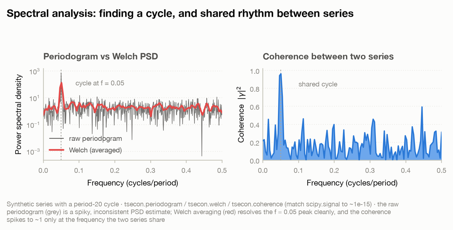The object it estimates is the power spectral density (PSD), the Fourier transform of the autocovariance function (Wiener-Khinchin), and its single most useful reading is direct — a peak in the PSD at frequency f is a cycle of period 1/f buried in the series. This family gives you three views. The raw periodogram is the one-FFT estimate: asymptotically unbiased but inconsistent, its variance never shrinks no matter how much data you add. Welch trades a little frequency resolution for a consistent, low-variance PSD by averaging periodograms over overlapping segments. And coherence is the frequency-domain analogue of a squared correlation between two series: at each frequency it asks how much of the two series' co-movement is shared at that cycle.

All three are one-sided, density-scaled estimators that match scipy.signal (periodogram, welch, coherence) to ~1e-15 in relative terms — the crate is a from-scratch Rust reimplementation pinned to the SciPy reference, not a wrapper. They share one input contract and two string knobs:

x  (and y)  : real 1-D arrays, sampled at rate fs (cycles per unit time)
returns     : freqs on [0, fs/2]  (one-sided, length nperseg//2 + 1)
window      : "boxcar" (no taper) or "hann" (the only two supported)
detrend     : "none" | "constant" (remove the mean) | "linear" (remove a line)

Two contract notes that bite in practice. First, the default detrend is "none", unlike SciPy's "constant" — a series with a nonzero mean or a trend will dump enormous power into the lowest-frequency bins and drown the cycles you are hunting, so pass detrend="constant" (or "linear") whenever x is not already zero-mean/detrended. Second, only "boxcar" and "hann" are recognized windows; anything else ("hamming", …) raises ValueError rather than being silently accepted.

---

periodogram — the one-FFT PSD estimate

What it estimates. The power spectral density of x from a single FFT of the whole (optionally windowed, optionally detrended) series: P(f_k) = |X(f_k)|^2 / (fs · Σ w_i^2), returned one-sided on the grid f_k = k·fs/n for k = 0 … n/2. It is the textbook periodogram of Schuster, density-scaled to match scipy.signal.periodogram(scaling="density"). The area under P approximates the variance of x; a tall narrow spike at f says a sinusoid of period 1/f is present.

Assumptions. A real, (weakly) stationary, evenly-sampled series. The estimate is asymptotically unbiased — each ordinate P(f_k) centres on the true spectral density S(f_k) as n grows — but it is not consistent: the variance of each ordinate stays of order S(f_k)^2 no matter how large n becomes (each P(f_k) behaves like S(f_k) times a χ²₂/2 variate). More data buys you a finer frequency grid, not a less noisy estimate at each frequency. That is the whole reason welch exists. A finite record also leaks power through the FFT's sidelobes, so a strong cycle bleeds into neighbouring bins — a Hann window suppresses that leakage at the cost of widening the main lobe.

When to use (and when not). Use it to detect the presence and location of a dominant periodicity — where is the peak, how sharp is it — and when you want the finest possible frequency grid from a short record and are willing to eyeball a spiky picture. Do not use the raw periodogram when you need a quantitative, low-variance PSD estimate (the height of any single ordinate is essentially one noisy draw): reach for welch. Do not run it on a series with a trend or nonzero mean without setting detrend — the leakage from the zero-frequency term will dominate everything.

Key arguments and defaults (and why). fs=1.0 sets the sampling rate and hence the frequency units (with fs=1, freqs runs 0 … 0.5 in cycles per sample and Nyquist is 0.5). window="boxcar" is no taper — SciPy's periodogram default, kept so leakage behaviour matches exactly; pass window="hann" to trade resolution for lower sidelobes. detrend="none" does nothing to the series; use "constant" to strip the mean or "linear" to strip a least-squares trend before the FFT. There is no segmenting knob — the periodogram is, by definition, one FFT over the entire input.

How to read the output. A dict with two equal-length arrays: freqs (0 … fs/2, length n//2 + 1) and psd (the density, non-negative everywhere). The peak location freqs[psd.argmax()] estimates the dominant cycle's frequency; 1/that is its period. Do not over-interpret the height of a single ordinate — it is high-variance.

Failure modes. Reading one PSD ordinate as a precise number — it is not, its sampling variance does not vanish with n. Forgetting to detrend, so a mean or trend swamps the low-frequency bins. Passing an unsupported window string (ValueError: unknown window …; expected "boxcar" or "hann") or detrend (ValueError: unknown detrend …). Expecting the peak to sit exactly on the true frequency — it lands in the nearest FFT bin, ±fs/2n away.

Validated against. scipy.signal.periodogram(detrend=False, scaling="density", window="boxcar"), stored as the golden fixture fixtures/spectral.json (generator fixtures/generate_spectral_fixtures.py) and checked in bindings/python/tests/test_spectral.py: freqs to atol 1e-10, psd to rtol 1e-8, atol 1e-12, with the non-negativity of the PSD asserted separately. The realized relative match on that fixture is ~1e-14.

References. Schuster (1898, Terrestrial Magnetism 3:13-41, the periodogram); Bartlett (1950, Biometrika 37:1-16, on its inconsistency); Percival & Walden (1993, Spectral Analysis for Physical Applications, Cambridge).

---

welch — segment-averaged, consistent PSD

What it estimates. Welch's (1967) averaged-periodogram PSD: split x into overlapping segments of length nperseg, window and periodogram each, then average the periodograms across segments. Averaging K roughly-independent segments cuts the sampling variance by about a factor of K (somewhat less with overlap, since overlapping segments are correlated), turning the periodogram's inconsistent estimate into a consistent one. The price is frequency resolution: with segments of length nperseg the frequency grid is spaced fs/nperseg, coarser than the full-length periodogram's fs/n.

Assumptions. The same real, stationary, evenly-sampled series — plus the stationarity has to hold across segments (Welch averages them as repeated looks at one spectrum, so a series whose spectral content drifts over the record violates the premise). Enough length to form several segments: nperseg ≤ n (a larger nperseg raises ValueError: segment length … exceeds the sample size …), and you want n comfortably larger than nperseg so the average is over more than a handful of segments.

When to use (and when not). This is the default choice whenever you want a PSD you can quantify rather than just a peak to eyeball — a smooth, reproducible spectrum whose ordinate heights mean something. The nperseg choice is the bias-variance dial: a long segment gives fine frequency resolution (sharp, well-separated peaks) but few segments to average, hence a noisier spectrum; a short segment averages many segments (smooth, low-variance) but blurs nearby peaks together and can bias a sharp line downward. Start around nperseg = n/8 and lengthen it if two peaks you care about are merging, shorten it if the spectrum is too ragged. Do not use Welch when the record is too short to segment meaningfully, or when you specifically need the finest grid a single FFT can give — use periodogram there.

Key arguments and defaults (and why). nperseg=256 is the segment length — the resolution/variance dial above. noverlap=None defaults to nperseg//2 (50% overlap), Welch's standard choice: with a Hann taper, 50% overlap recovers most of the data that windowing down-weights near the segment edges, so successive segments stay nearly uncorrelated while wasting little of the record. window="hann" is the default taper (SciPy's), because averaging many segments makes leakage suppression matter more than main-lobe width; "boxcar" is available for an untapered average. fs and detrend behave exactly as for periodogram.

How to read the output. A dict of two arrays: freqs (0 … fs/2, length nperseg//2 + 1) and psd. The spectrum is smoother and shorter than the periodogram's; the peak freqs[psd.argmax()] still estimates the dominant cycle, now with a stable, interpretable height. On a log-y axis a broadband noise floor plus a clean spike at the cycle frequency is the canonical picture.

Failure modes. Setting nperseg too large — few segments, a spectrum barely less noisy than the raw periodogram, or nperseg > n which raises. Setting it too small — a heavily smoothed spectrum that merges distinct peaks and underestimates a sharp line's height. Averaging over a series whose spectrum is non-stationary (the segments are not repeated looks at one spectrum). Omitting detrend on a trending series.

Validated against. scipy.signal.welch(nperseg=128, detrend=False, scaling="density"), golden fixture fixtures/spectral.json, checked in bindings/python/tests/test_spectral.py (freqs to atol 1e-10, psd to rtol 1e-8, atol 1e-12). The realized relative match on that fixture is ~1e-15.

References. Welch (1967, IEEE Transactions on Audio and Electroacoustics 15:70-73); Percival & Walden (1993, Spectral Analysis for Physical Applications, Cambridge); Priestley (1981, Spectral Analysis and Time Series, Academic Press).

import numpy as np, tsecon

rng = np.random.default_rng(7)
n = 1024
t = np.arange(n)
period = 20.0                                   # one cycle every 20 samples => f = 0.05
x = 1.5 * np.sin(2 * np.pi * t / period) + rng.standard_normal(n)

pg = tsecon.periodogram(x, window="boxcar", detrend="none")   # one FFT, high variance
wl = tsecon.welch(x, nperseg=256, detrend="none")             # segment-averaged, smoother
fp, psd_p = np.asarray(pg["freqs"]), np.asarray(pg["psd"])
fw, psd_w = np.asarray(wl["freqs"]), np.asarray(wl["psd"])

print(f"true cycle frequency        : {1/period:.3f}  (period {period:.0f} samples)")
print(f"periodogram peak frequency  : {fp[psd_p.argmax()]:.4f}   ({len(fp)} freq bins)")
print(f"Welch       peak frequency  : {fw[psd_w.argmax()]:.4f}   ({len(fw)} freq bins)")

off = lambda f, p: p[(f > 0.20) & (f < 0.45)].std()   # roughness away from the peak
print(f"off-peak PSD std, periodogram: {off(fp, psd_p):.3f}")
print(f"off-peak PSD std, Welch      : {off(fw, psd_w):.3f}   (averaging cuts the variance)")

from scipy import signal                            # one-line parity cross-check
_, psd_sp = signal.welch(x, nperseg=256, detrend=False, scaling="density")
print(f"max |Welch - scipy.signal|   : {np.max(np.abs(psd_w - psd_sp)):.1e}")
# true cycle frequency        : 0.050  (period 20 samples)
# periodogram peak frequency  : 0.0498   (513 freq bins)
# Welch       peak frequency  : 0.0508   (129 freq bins)
# off-peak PSD std, periodogram: 1.615
# off-peak PSD std, Welch      : 0.655   (averaging cuts the variance)
# max |Welch - scipy.signal|   : 2.8e-14

Both estimators put the peak on the period-20 cycle (f ≈ 0.05), so either one finds the cycle. The difference is everywhere else: the raw periodogram has 513 noisy ordinates whose off-peak scatter is 1.615, while Welch's 128-fold averaging (fewer, coarser bins) drops the off-peak scatter to 0.655 — a quieter, quantifiable spectrum. And the Welch PSD reproduces scipy.signal.welch to ~1e-14, confirming the from-scratch estimator is the SciPy quantity to machine precision.

---

coherence — shared rhythm between two series

What it estimates. The magnitude-squared coherence between x and y, C_xy(f) = |S_xy(f)|² / (S_xx(f) · S_yy(f)), computed from Welch-averaged auto- and cross-spectra. It is the frequency-domain analogue of a squared correlation coefficient, lying in [0, 1] at every frequency: C_xy(f) ≈ 1 means the two series' variation at cycle f is (up to a linear filter / phase shift) perfectly shared, C_xy(f) ≈ 0 means their fluctuations at that cycle are unrelated. It answers "at which frequencies do these two series move together?" — a question a single time-domain correlation cannot resolve.

Assumptions. Two real, jointly stationary, evenly-sampled series of equal length (unequal lengths raise ValueError: cross-spectral inputs differ in length …). Critically, coherence must be estimated by averaging over segments: with a single segment the cross-spectrum and the two auto-spectra collapse so that the ratio is identically 1 at every frequency — a degenerate, meaningless result. So nperseg has to be small enough (relative to n) that several segments are averaged; the more segments, the lower the variance of the coherence estimate and the smaller its upward small-sample bias.

When to use (and when not). Use it to ask whether two series share a specific cyclical component — a common business-cycle frequency across two macro aggregates, a shared seasonal, a lead-lag relationship that operates only at certain periods — rather than a single scalar "are they correlated?" It is not a causality or a direction test: coherence is symmetric in x and y and says nothing about which leads (that information is in the cross-spectrum's phase, which this function does not return). And it is not a substitute for averaging — with too few segments the estimate biases toward 1.

Key arguments and defaults (and why). Same segmenting surface as welch: nperseg=256, noverlap=None (→ nperseg//2, 50%), window="hann", plus fs and detrend. The one extra design consideration is that nperseg now has a hard statistical floor as well as ceiling — pick it small enough that n/nperseg gives you several segments, or the coherence is trivially 1.

How to read the output. A dict with freqs (0 … fs/2) and coherence (each entry in [0, 1]). Scan for frequencies where coherence rises toward 1: those are the cycles the two series share. Low coherence at a frequency where one series has a strong spectral peak means that peak is private to that series.

Failure modes. Using too few segments (large nperseg relative to n), which biases coherence toward 1 — the single-segment limit is identically 1. Reading coherence as directional or causal (it is symmetric; phase carries the lead-lag). Feeding mismatched-length series (raises). Forgetting detrend when a shared trend would inflate low-frequency coherence spuriously.

Validated against. scipy.signal.coherence(nperseg=128, detrend=False), golden fixture fixtures/spectral.json, checked in bindings/python/tests/test_spectral.py (coherence to rtol 1e-8, atol 1e-10, with the [0, 1] bound asserted). The realized match on that fixture is ~1e-16.

References. Carter, Knapp & Nuttall (1973, IEEE Transactions on Audio and Electroacoustics 21:337-344, estimation of magnitude-squared coherence); Percival & Walden (1993, Spectral Analysis for Physical Applications, Cambridge); Brockwell & Davis (1991, Time Series: Theory and Methods, 2nd ed., Springer).

import numpy as np, tsecon
from scipy import signal

rng = np.random.default_rng(11)
n = 2048
t = np.arange(n)
shared = np.sin(2 * np.pi * 0.02 * t)               # a slow cycle both series share
x = shared + 0.8 * rng.standard_normal(n)
y = 0.9 * shared + np.sin(2 * np.pi * 0.15 * t) + 0.8 * rng.standard_normal(n)  # y also has a PRIVATE cycle

co = tsecon.coherence(x, y, nperseg=256, detrend="none")   # 2048/256 -> several segments to average
fc, coh = np.asarray(co["freqs"]), np.asarray(co["coherence"])
at = lambda f0: coh[np.abs(fc - f0).argmin()]

print(f"coherence at f=0.02 (shared) : {at(0.02):.3f}   -> near 1: series move together here")
print(f"coherence at f=0.15 (y only) : {at(0.15):.3f}   -> near 0: no shared power there")
print(f"coherence stays in [0, 1]    : [{coh.min():.3f}, {coh.max():.3f}]")

_, coh_sp = signal.coherence(x, y, nperseg=256, detrend=False)
print(f"max |coherence - scipy|      : {np.max(np.abs(coh - coh_sp)):.1e}")
# coherence at f=0.02 (shared) : 0.955   -> near 1: series move together here
# coherence at f=0.15 (y only) : 0.001   -> near 0: no shared power there
# coherence stays in [0, 1]    : [0.000, 0.955]
# max |coherence - scipy|      : 3.3e-16

The two series share one slow cycle (f = 0.02) and y carries a second cycle (f = 0.15) that x does not. Coherence reads this correctly: it rises to 0.955 at the shared frequency and sits at 0.001 at y's private one — a distinction no single time-domain correlation could draw. The estimate never leaves [0, 1], and it reproduces scipy.signal.coherence to ~1e-16.